Now here is a small exercise to get a feeling for that p < 5% figure … are your coins really fair?
Choose a coin, any coin.
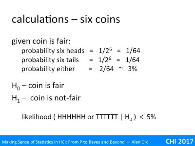
If a coin is fair then the probability of six heads is 1/64 as is the probability of six tails, and the probability of six of either is 2/64, approximately 3%.
So we can do an experiment.
H0 the null hypothesis is that the coin is fair.
H1 the alternative hypothesis is that the coin is not fair.
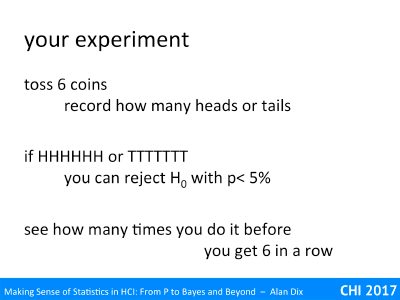
The likelihood of HHHHHH or TTTTTT given H0 is less than 5%, so if you get six heads or six tails, you can reject the null hypothesis and conclude that the coin is not fair.
Try it, and if it doesn’t work try again. How long before you end up with a ‘statistically significant’ test?
Think back to the discussion of cherry picking and multiple tests …
This might seem a little artificial, but imagine rather than coin tossing it is six users preferences for software A or B.
Having done this, how do you feel about whether 5% is a suitable level to regard as evidence?
This is the point where I nail my colours to the mast – should you use traditional statistics or Bayesian methods? With all the controversy in the media about the ‘statistical crisis’ should one opt for alt-stats or stay with conservative ones? Of course the answer will partly be ‘it depends’, but for most purposes I think there is a best answer …
You may have seen stories about the ‘statistical crisis’ [Ba16]. A variety of papers and articles in the technical and sometimes even popular press highlighting general poor statistical practice. This has touched many disciplines, including HCI [Ca07, KN16].
Some have focused on the ‘replication crisis’, the fact that many attempts to repeat scientific studies have failed to reproduce the original (often statistically significant) outcomes. Other have focused on the statistics itself, especially p-hacking, where wittingly or unwittingly scientists use various means to ensure they get the necessary p<5% to enable them to publish their results.
Some of these problems are intrinsic to the scientific publishing process.
One is the tendency for journals to only accept positive results, so that non-significant results do not get published. This sounds reasonable until you remember that the p<5% means that on average one time in twenty you reject the null hypothesis (appear to have a positive finding) by shear chance. So if 100 scientists do experiments where there is no real effect, typically this will lead to 5 apparently ‘publishable’ effects.
Another problem is that the ‘publish or perish’ culture of academia means that researchers may ‘bend’ the facts slightly to get publishable results. To be fair this may be because they are convinced for other reasons that something is true, so they ‘gild the lily’ a little, ignoring negative indications and emphasising positive ones. As we saw previously, famous scientists have done this in the past, and because what they did happened to be true history has overlooked the poor stats (or looked the other way).
Most of the publicity on this has focused on traditional hypothesis testing. However, the potential problems in traditional statistics have been well known for at least 40 years and are to do with poor use or poor interpretation, not intrinsic weaknesses in the statistical techniques themselves.
There have been some changes, which may have led to the current level of publicity. One is the increasing publication pressures mentioned above. Another is that in years gone by when scientists needed to do statistics they would typically ask a statistician for advice, especially if it was at all unusual or unlike previous studies. Indeed, my own first job was at an agricultural engineering research institute, where, in addition to my main role doing mathematical and computational modelling, I was part of the institute’s statistics advisory team. Now time and budgetary constraints mean that research institutions are less likely to offer easy access to statistical advice and instead researchers reach for easy to use, but potentially easy to misuse, statistical packages.
However, there is also not a little hype amongst the genuine concern, including some fairly shaky statistical methods in some of the papers criticising statistical methods!
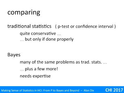
Most of the ‘bad press’ has focused on traditional statistics and in particular hypothesis testing – the dreaded p! As noted, this is largely due to well-understood issues when they are used inexpertly or badly. When used properly, traditional statistics (both hypothesis testing and confidence intervals) tend to be relatively conservative.
One reaction to this has been for some to abandon statistics entirely; famously (or maybe infamously) the journal Basic and Applied Social Psychology has banned all hypothesis testing [Wo15]. However, this is a bit like getting worried about the safety of a cruise ship sinking and so jumping into the water to avoid drowning. The answer to poor statistics is better statistics not no statistics!
The other reaction has been to loom to alternative statistics or ‘new statistics’; this has included traditional confidence intervals and also Bayesian statistics. Some of this is quite valid; the good use of statistics includes using the correct type of analysis for the kinds of data and information you have available. However, the advocacy of these alternatives can sometimes include an element of snake oil (paper titles such as “Using Bayes to get the most out of non-significant results” probably don’t help [Di14]).
Crucially, most of the problems that have been identified in the ‘statistical crisis’ also apply to alternative methods: selective publication, p-hacking (or various other forms of cherry picking), post-hoc hypotheses. In addition, reduced familiarity can lead to poorer statistical execution and reporting. Bayesian statistics in particular currently requires considerable expertise to be used correctly. Indeed, at the time of writing the Wikipedia page for Bayes Factor (Bayesian alternative to hypothesis testing) includes, as its central example, precisely this kind of inexpert use of the methods [W17].
There are good reasons why, even after 40 plus years of debate, most professional statisticians still use traditional methods!
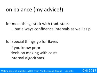
Based on all this my personal advice is that for most things stick with traditional statistics, but where possible always quote confidence intervals alongside any form of p-value (APA also recommend this [AP10]).
This is partly because, despite the potential misuse, there is still better general understanding of these methods and their pitfalls. You are more likely to do them right and your readers are more likely to have an idea of what they mean.
This said there are a number of circumstances when Bayesian statistics are not only a good idea, but the only sensible thing to do. These are usually circumstances where you know the prior and are involved in some sort of decision-making. For example, if a patient is in hospital you know the underlying prevalence of various diseases and so should use this as part of diagnostic reasoning. This also applies in the algorithmic use of Bayesian methods in intelligent or adaptive interfaces.
If you do choose to use Bayesian statistics, do ensure you consult an expert, especially if you are dealing with continuous values (such as completion times), as the theory around these is particularly complex (is is evident on the Wikipedia page!). Do be careful to that your prior is not simply meaning you are confirming your own bias. Also do be aware that the odds ratios that are taken as acceptable evidence seem (to a traditional statistician!) to be somewhat lax (and 5% sig. is already quite lax!), so I would advise using one of the more strict levels.
Whether you use traditional stats, p-values, confidence intervals, Bayesian statistics, or tea-leaf reading – make sure you use the statistics properly. Understand what you are doing and what the results you are presenting mean.
… and I hope this course helps!
Endnote
For a balanced view of Bayesian methods see the interview with Peter Diggle, President of the Royal Statistical Society [RS15]. However, it is perhaps telling that the Royal Statistical Society’s own mini-guide for non-statisticians, also called ‘Making Sense of Statistics”, avoids mentioning Bayesian methods entirely [SS10].
References
[AP10] APA (2010). Publication Manual of the American Psychological Association, Sixth Edition. http://www.apastyle.org/manual/
[Ba16] Baker, M. (2016). Statisticians issue warning over misuse of P values. Nature, 531, 151 (10 March 2016) doi:10.1038/nature.2016.19503
[Ca07] Paul Cairns. 2007. HCI… not as it should be: inferential statistics in HCI research. In Proceedings of the 21st British HCI Group Annual Conference on People and Computers: HCI…but not as we know it – Volume 1 (BCS-HCI ’07), Vol. 1. British Computer Society, Swinton, UK, UK, 195-201.
[Di14] Dienes, Z. (2014). Using Bayes to get the most out of non-significant results. Frontiers in Psychology, 5, 781. http://doi.org/10.3389/fpsyg.2014.00781
[KN16] Kay, M., Nelson, G., and Hekler, E. 2016. Researcher-Centered Design of Statistics: Why Bayesian Statistics Better Fit the Culture and Incentives of HCI. CHI 2016, ACM, pp. 4521-4532.
[RS15] RSS (2015). Statistician or statistical scientist? an interview with RSS president Peter Diggle. StatsLife, Royal Statistical Society. 08 January 2015. https://www.statslife.org.uk/features/2822-statistician-or-statistical-scientist-an-interview-with-rss-president-peter-diggle
[SS10] Sense about Science (2010). Making Sense of Statistics. Sense about Science. in collaboration with the Royal Statistical Society. 29 April 2010. http://senseaboutscience.org/activities/making-sense-of-statistics/
[W17] Wikipedia (2017). Bayes factor. Wikipedia. Internet Archive at 26th July 2017. https://web.archive.org/web/20170722072451/https://en.wikipedia.org/wiki/Bayes_factor
[Wo15] Chris Woolston (2015). Psychology journal bans P values. Nature News, Research Highlights: Social Selection. 26 February 2015. http://www.nature.com/news/psychology-journal-bans-p-values-1.17001
Many statistical tests depend on the idea of outcomes that are the same or worse than the one you have observed. For example, if you have the difference in response times between two systems is 5.7 seconds, then 5.8, 6, 23 seconds are all ‘the same or worse’, equally or more surprising. For numeric values this is fairly straightforward, but can be more complex when looking at different sorts of patterns in data. This is critical when you are making ‘post-hoc hypotheses’, noticing some pattern in the data and then trying to verify whether it is a real effect or simple chance.
You have got hold of the stallholder’s coin and wondering if it is fair or maybe weighted in some way.
Imagine you toss it 10 times and get the sequence: THTHHHTTHH
Does that seem reasonable?
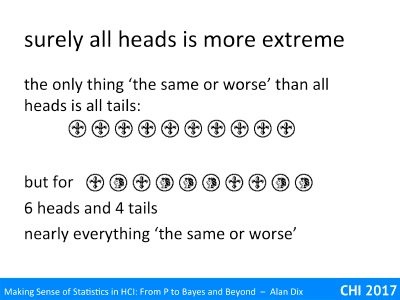
What about all heads? HHHHHHHHHH
In fact, if the coin is fair the probability of any sequence of heads and tails is the same: 1 in 1024
Prob( THTHHHTTHH ) = 1/ 210 ~ 0.001
Prob( HHHHHHHHHH ) = 1/ 210 ~ 0.001
The same would be true of a pack of cards. There are 52! Different ways a pack of cards can come out (Note. 52! Is 52 factorial, the product of all the numbers up to 52 = 52x51x50 … x3x2x1), approximately the number of atoms in our galaxy. Each order is equally likely on a wells shuffled pack, so any pack you pick up is incredibly unlikely.
However, this goes against our intuition that some orders of cards, some patterns of coin tosses are more special than others.
This is where we need to have an idea of things that are similar or equally surprising to each other.
For the line of 10 heads, the only thing equally surprising would be a line of 10 tails. However for the pattern THTHHHTTHH, with 6 heads and 4 tails in a pretty unsurprising order (not even all the heads together), pretty much any other order s equally or more surprising, indeed if you are thinking about a fair coin, arguably the only thing less surprising is exactly five of each.
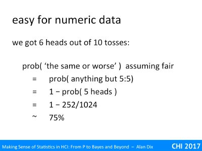
This idea of same or worse is relatively straightforward for numeric data such as completion time in an experiment, or number of heads in coin tosses.
We got 6 heads out of 10 tosses, so that 6, 7, 8, 9, 10 heads would be equally or more surprising, as would 6,7,8,9,10 tails.
So yes, 9 heads is starting to look more surprising, but is it enough to call the stallholder out for cheating?
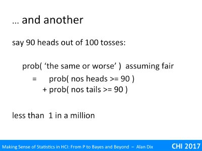
As a final example, imagine 90 heads out of 100 tosses – the same proportion, but more tosses, therefore you expect things to ‘average out’ more.
Here the things that are equally or more surprising are 90 or more heads or 90 or more tails.
prob ( ‘the same or worse’ ) assuming fair
= prob ( nos heads >= 90 ) + prob ( nos tails >= 90 )
less than 1 in a million
The maths for this gets a little more complicated, but turns out to be less than one in a million. If this were a Wild West film this is the point the table would get flung over and the shooting start!
For continuous distributions, such as task completion times, the principle is the same. The maths to work out the probabilities gets harder still, but here you just look up the numbers in a statistical table, or rely on R or SPSS to wok it out for you.
For example, you measure the average task completion time for ten users of system A as 117.3 seconds and for ten users of system B it is 98.1 seconds. On average for the participants in your user test system B was 18.2 seconds faster. Can you conclude that your newly designed system B is indeed faster to use?
Just as with the coin tosses, the probability of a precisely 18.2 second difference is vanishingly small, it could be 18.3 or 18.1, or so many possible values. Indeed, even if the systems were identical, the probability of the difference being precisely zero, or 0.1 seconds, or 0.2 seconds are all still pretty tiny. Instead you look at the probability (given the systems are the same) that the difference is 18.2 or greater.
For numeric values, the only real complication is whether you want a one or two tailed test. In the case of checking whether the coin is far, you would be equally upset if it had been weighted in some way in either direction, hence you look at both sides equally and work out (for the 90 heads out of 100): prob (nos heads >=90) + prob( nos tails >= 90).
However, for the response time, you probably only care about your new system being faster than the old one. So in this case you would only look at the probability of the time difference being >=18.2, and not bother about it being larger in the opposite direction.
Things get more complex in various forms of combinatorial data, for example, friendship circles in network data. Here what it means to be the ‘same or worse’ can be far more difficult.
As an example of this kind of complexity, we’ll return to playing cards. Recall as many ways to shuffle the pack as atoms in the galaxy.
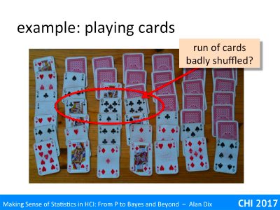
I sometimes play a variety of ‘patience’ (a solitaire card game) which involves laying out a 7×7 grid with the lower left triangle exposed and the upper right face down.
One day I was dealing these out and noticed that three consecutive cards had been jack of clubs, 10 of clubs, 9 of clubs.
My first thought was that I had not shuffled the cards well and this pattern was due to some systematic effects from a previous card game. However, I then realised that the previous game would not lead to sequences of cards in suit.
So what was going on? Remembering the rain drops in the Plains of Nali, is this chance or an omen?
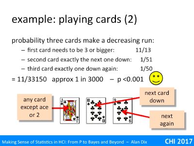
Let’s look a little more closely. If you deal three cards in a row, what is the probability it will be a decreasing sequence?
Well, the first card can be anything except an ace or a 2, that is 44 out of 52 cards, or 11/13.
After this the second and third cards are precisely determined by the first card, so have probability of 1/51 and 1/50 respectively.
Overall the probability f three cards being in a downward run in suit is 11/33350, or about 1 in 3000 … pretty unlikely and if it were doing statistics after a usability experiment you would get pretty excited with p <0.0001
However, that is not the end of the story. I would have been equally surprised if it had been an ascending, or if the run had been anywhere amongst the visible cards where there are 15 possible start positions for a run of three. So, our probability of it being a run up or down in any of these start positions is now 30 x 11 / 33350 or about 1 in a 100.
But then there are also vertical runs up and down the cards, or perhaps runs of the same number from different suits that would also be equally surprising.
Finally how many times do I play the game? I probably only notice when there is something interesting (cherry picking), suddenly my run of three does not looks so surprising.
In some ways noticing the jack, ten, nine run was a bit like a post-hoc hypothesis.
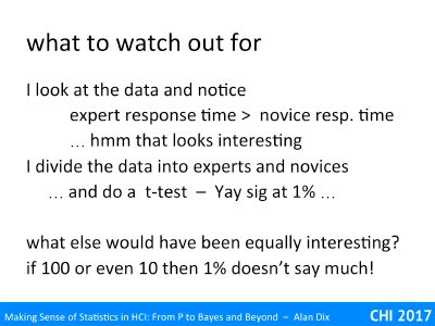
You have run your experiment, looked at the data and the notice that it looks as though expert response time is slower than novice response time. This looks interesting, so you follow this up with a formal statistical test. You divide the data into novice and expert calculate averages, do the sums and and it comes out significant at 1%.
Yay, you have found out something … or have you?
What else would have been equally interesting that you might have noticed, age effects, experience, exposure to other kinds of software, those wearing glasses vs. those with perfect visions?
Remember your Bonferroni correction, if there are 10 things that would have been equally surprising, your 1% statistical significance is really only equivalent to 10%, which may be just plain chance.
Think back to the raindrops patterns on the Plain of Nali. One day’s rainfall included three drops is an almost straight line, but turned out to be an entirely random fall pattern. You notice the three drops in a line, but how many lots of three are there, how close to a line before you call it straight? Would small triangles, or squares have been equally surprising.
In an ideal (scientific) world, you would use patterns you notice in data as hypotheses for a further round of experiments … but often that is not possible and you need to be able to both spot patterns and make tests on their reliability on the same data.
One way to ease this is to visualise a portion of the data and then check it on the rest – this is similar to techniques used in machine earning. However, again that may not always be possible.
So, if you do need to make post-hoc hypotheses, try to make an assessment of what other things would ‘similar or more surprising’ and use this to help decide whether you are just seeing random patterns in the wild-slung stars.
Traditional statistics and Bayesian methods have their own specific pitfalls to avoid: for example interpretation of non-significant as no effect in traditional stats and confirmation bias for Bayesian stats.
They also have some common potential pitfalls. Perhaps the worst is cherry picking – doing analysis using different tests, and statistics, and methods until you find one that ‘works’! You also have to be careful of inter-related factors such as the age and experience of users. By being aware of these dangers one can hopefully avoid them!
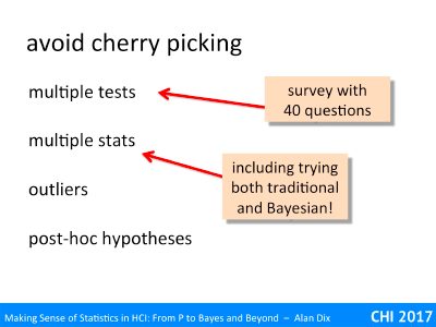
One of the most common problems in statistics are forms of ‘cherry picking’, this is when you ignore results that for some reason are not to your liking and instead just report those that are advantageous. This may be a deliberate attempt to deceive, but more commonly is simply a combination of ignorance and bias. In hypothesis testing people talk about ‘p=hacking’, but this can equally be a problem for Bayesian statistics or confidence intervals.
multiple tests
The most obvious form of cherry picking is when you test loads and loads of things and then pick out the few that come out showing some effect (p value or odds ratio) and ignoring the rest, or even worse the few that come out showing the effect you want and ignoring the ones that point the opposite way!
A classic example of this is when you have a questionnaire administered after a user test, or remotely. You have 40 questions comparing two versions of a system (A and B) in terms of satisfaction, and the questions cover different aspects of the system and different forms of emotional response. Most of the questions come out mixed between the two systems, but three questions seem to show a marked preference for the new system. You then test these using hypothesis testing and find that all three are statistically significant at 5% level. You report these and feel you have good evidence that system B is better.
But hang on, remember the meaning of 5% significance is that there is a 1 in 20 chance of seeing the effect by sheer chance. So, if you have 40 questions and there is no real difference, then would you might expect to see, on average, 2 hits at this 1 in 20 level, sometimes just 1, sometimes 3 or more. In fact there is an approximately one in three chance that you will have 3 or more apparently ‘5% significant’ results with 40 questions.
The answer to this is that if you would have been satisfied with a 5% significance level for a single test and have 10 tests, then any single one needs to be at the 0.5% significance level (5% / 10) in order to correct for the multiple tests. If you have 40 questions, this means we should look for 0.125% or p<0.00125.
This dividing the target p level by the number of tests is called the Bonferroni correction. It is very slightly conservative and there are slightly more exact versions, but for most purposes this is sufficiently accurate..
multiple stats
A slightly less obvious form of cherry picking is when you try different kinds of statistical technique. First you try a non-parametric test, then a t-test, etc., until something comes out right.
I have seen one paper where all the statistics were using traditional hypothesis testing, and then in the middle there was one test that used Bayesian statistics. There was no explanation and my best bet was they the hypothesis testing had come out negative so they had a go with Bayesian and it ‘worked’.
This use of multiple kinds of statistics is not usually quite as bad as testing lots of different things as it is the same data so the test are not independent, but if you decide to swop the statistics you are using mid-analysis, you need to be very clear why your are doing it.
It may be that you have realised that you were initially using the wrong test, for example, you might have initially used a test, such as Student’s t, that assumes normally distributed data, but only after starting the analysis realise this is not true of the data. However, simply swopping statistics part way through in the hope tat ‘something will come out’ is just a form of fishing expedition!
For Bayesian stats the choice of prior can also be a form of cherry picking if you try one and then another, until you get the result you want.
outliers
A few outliers, that is extreme values, can have a disproportionate effect on some statistics, notably arithmetic mean and variance. They may be due to a fault in equipment, or some other irrelevant effect, or may simply occur by chance.
If they do appear to be valid data points that just happen to be extreme, there is an argument for just letting them be as they are part of the random nature of the phenomenon you are studying. However, for some purposes, one gets better results by removing the most extreme outliers.
However, this can add a cherry picking potential. Ne of the largest effects of removing outliers is to reduce the variance of the sample, and a large sample variance reduces the likelihhod of getting a statistically significant effect, so there is a temptation to strip out outliers until the stats come out right.
Ideally you should choose a strategy for dealing with outliers before you do your analysis. For example, some analysis choose to remove all data that lies more than 2 or 3 standard deviations from the mean. However, there are times when you don’t realise outliers are likely to be a problem until they occur. When this happens you should attempt to be as blind to the stats as possible as you choose which outliers to remove, do avoid removing a few re-testing, removing a few more then re-testing again!
post-hoc hypothesis
The final kind of cherry picking to beware of is post-hoc hypothesis testing.
You gather your data, visualise it (good practice), and notice an interesting pattern, perhaps a correlation between variables and then test for it.
This is a bit like doing multiple test, but with an unspecified number of alterative tests. For example, if you have 40 questions, then there are 780 different possible correlations, so if you happen to notice one and then test for it, this is a bit like doing 780 tests!
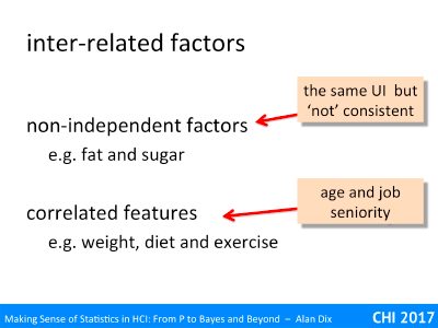
Another potential danger is where the factors you are trying to control for or measure are in some way inter-related making it hard to interpret results, especially potential causes for observed effects.
non-independently controllable factors
Sometimes you cannot change one parameter without changing others as well.
For example, if you are studying diet and try to reduce sugar intake, then it is likely that either fat intake will go up to compensate or overall calorie intake will fall. You can’t reduce sugar without something else changing.
This often happens with user interface properties or features.
For example imagine you find people are getting confused by the underline option on a menu, so you change it so the menu item says ‘underline’ when the text is not underlined, and ‘remove underline’ when it is already underlined. This may improve the underline feature, but then maybe users are confused because it still says ‘italic’ when the selected text is already italicised.
Similarly, imagine trying to take a system and make a version that is ‘not consistent’ but otherwise identical. In practice once you change one things, you need to change many others to make a coherent design.
The effect fo this is that you cannot simply say, in the diet example “reducing sugar has this effect”, but instead it is more likely to be “reducing sugar whilst keeping the rest of the diet fixed 9and hence reducing calories …” or “reducing sugar whilst keeping calorie intake constant (and hence probably increasing fact) …”.
In the menu example, you probably can’t just study the effects of the underline / remove underline menu options without changing all menu items, and hence will e studying constant name vs. state-based action naming, or something like that.
correlated features
A similar problem can occur with features of you users which you cannot directly control at all.
Let’s start again with a dietary example. Imagine you have clinical measures of health, perhaps cardiovascular tests results, and want to work out what factors in day-to-day life contribute to health, so you administer a life-style questionnaire. One question is about the amount of exercise they take and you find this correlates positively with cardio-vascular health, that s good. However, it maybe that someone who is a little overweight is less likely to take exercise, or vice versa. The different lifestyle traits: healthy diet, weight, exercise are likely to be correlated and thus it can be difficult to disentangle which are the casual factors for measured effects.
In a user interface setting we might have found that more senior managers work best with slightly larger fonts than their juniors. Maybe you surmise that this might be something to do with the high level of multi-tasking and the need for ‘at a glance’ information. However, on the whole those in more senior positions tend to be older than those in more junior positions, so that the preference is more to do with age-related eyesight problems.
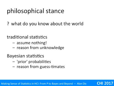
Although they are both founded in probability theory, traditional statistics and Bayesian statistics have fundamental philosophical differences in the way they treat uncertainty. Bayesian methods demand the uncertainty is quantified, whereas traditional methods accept this uncertainty and reason form that. However, in practice our knowledge is somewhere between complete ignorance and precise probability, and both methods have ways of dealing with this in-between knowledge.
We have seen that both traditional statistics and Bayesian statistics effectively start with the same underlying data, and in many circumstances yield effectively equivalent results. However, they adopt fundamentally different philosophical stance in the way that they sue that data to answer questions about the world. These philosophical differences are critical in interpreting their results.
Traditional statistics effectively assumes nothing about the world: are there Martians or not, is your new design better than the old one or not, it is not so much neutral as takes no sides at all. It then seeks to reason from that state of unknowledge.
Bayesian statistics instead asks you to quantify that unknowledge into prior probabilities, and then reasons in an apparently mathematically clean way, but based on those guestimates.
In some ways traditional statistics is post-modern accepting uncertainty and leaving it even in the eventual interpretation of the results, whereas Bayesian statistics suggest a more closed world. However, with Bayesian stats the uncertainty is still there, just encapsulated in the guestimate of the prior.
On the surface they have radically different assumtoiosn about the unknown features of the real world. Traditional statistics assumes no knowledge of the real value, whereas Bayesian statistics assumes a precise porbailty dustriution.
However, neither the world, not the statistics we use to make sense of it, are as clear-cut.
Typically we have some knowledge about the likelihood (in the day to day sense) of things: you are pretty unlikely to encounter Martians; the coin you’ve pulled from your pocket is likely to be fair; that new design for the software, you’ve put a lot of effort into creating should be better than the old system. However, typically we do not have a precise measure of that knowledge.
In their purest form traditional statistics entirely ignores that knowledge and Bayesian statistics asks you to make it precise in a way that goes beyond you actual knowledge, turning uncertainty into precise probability. The former ignores information, the latter forces you to invent it!
In practice, both techniques are a little more nuanced.
In traditional statistics the significance level you are willing to accept as good evidence (p<5%, p<1%) often reflects your prior beliefs: you will probably need a very high level before you really call the Men in Black, or even accept that the coin may be loaded. Effectively there is a level of Bayesian reasoning applied during interpretation.
Similarly, while Bayesian statistics demands a precise prior probability distribution, in practice often uniform or other forms of very ‘spread’ priors are used, reflecting the high degree of uncertainty. Ideally it would be good to try a number of priors to obtain a level sensitivity analysis, rather as we did in the example, but I have not seen this done in practice., possibly as it would add another level of interpretation to explain!
Bayesian reasoning allows one to make strong statements about the probability of things based on evidence. This can be used for internal algorithms, for example, to make adaptive or intelligent interfaces, and also for a form of statistical reasoning that can be used as an alternative to traditional hypothesis testing.
However, to do this you need to be able to quantify in a robust and defensible manner what are the expected prior probabilities of different hypothesis before an experiment. This has potential dangers of confirmation bias, simply finding the results you thought of before you start, but when there are solid grounds for those estimates it is precise and powerful.
Crucially it is important to remember that Bayesian statistics is ultimately about quantified belief, not probability.
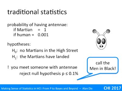
It is common knowledge that all Martians have antennae (just watch a sci-fi B-movie). However, humans rarely do. Maybe there is some rare genetic condition or occasional fancy dress, so let’s say the probability that a human has antennae is no more than 1 in a 1000.
You decide to conduct a small experiment. There are two hypotheses:
H0 – there are no Martians in the High Street
H1 – the Martians have landed
You go out into the High Street and the first person you meet has antennae. The probability of this occurring given the null hypothesis that there are no Martians in the High Street is 1 in 1000, so we can reject the null hypothesis at p<=0.1% … which is a far stronger result than you likely to see in most usability experiments.
Should you call the Men in Black?
For a more familiar example, let’s go back to the coin tossing. You pull a coin out of your pocket, toss it 10 times and it is a head every time. The chances of this given it is a fair coin is just 1 in 1000; do you assume that the coin is fixed or that it is just a fluke?
Instead imagine it is not a coin from your pocket, but a coin from a stall-holder at a street market doing a gambling game – the coin lands heads 10 times in a row, do you trust it?
Now imagine it is a usability test and ten users were asked to compare your new system that you have spent many weeks perfecting with the previous system. All ten users said they prefer the new system … what do you think about that?
Clearly in day-to-day reasoning we take into account our prior beliefs and use that alongside the evidence from the observations we have made.
Bayesian reasoning tries to quantify this. You turn that vague feeling that it is unlikely you will meet a Martian, or unlikely the coin is biased, into solid numbers – a probability.
Let’s go back to the Martian example. We know we are unlikely to meet a Martiona, but how unlikely. We need to make an estimate of this prior probability, let’s say it is a million to one.
prior probability of meeting a Martian = 0.000001
prior probability of meeting a human = 0.999999
Remember that the all Martians have antennae so the probability that someone we meet has antennae given they are Martian is 1, and we said the probability of antennae given they are human was 0.001 (allowing for dressing up).
Now, just as in the previous scenario, you go out into the High Street and the first person you meet has antennae. You combine this information, including the conditional probabilities given the person is Martian or human, to end up with a revised posterior probability of each:
posterior probability of meeting a Martian ~ 0.001
posterior probability of meeting a human ~ 0.999
We’ll see and example with the exact maths for this later, but it makes sense that if it were a million times more likely to meet a human than a Martian, but a thousand times less likely to find a human with antennae, then about having a final result of about a thousand to one sounds right.
The answer you get does depend on the prior. You might have started out with even less belief in the possibility of Martians landing, perhaps 1 in a billion, in which case even after seeing the antennae, you would still think it a million times more likely the person is human, but that is different from the initial thousand to one posterior. We’ll see further examples of this later.
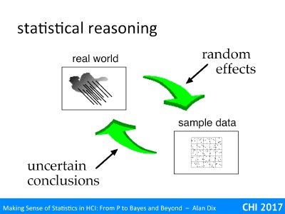
So, returning once again to the job of statistics diagram, Bayesian inference is doing the same thing as other forms of statistics, taking the sample, or measurement of the real world, which includes many random effects, and then turning this back to learn things about the real world.
The difference in Bayesian inference is that it also asks for a precise prior probability, what you would have thought was likely to be true of the real world before you saw the evidence of the sample measurements. This prior is combined with the same conditional probability (likelihood) used in traditional statistics, but because of the extra ‘information’ the result is a precise posterior distribution that says precisely how likely are different values or parameters of the real world.
The process is very mathematically sound and gives a far more precise answer than traditional statistics, but does depend on you being able to provide that initial precise prior.
This is very important, if you do not have strong grounds for the prior, as is often the case in Bayesian statistics, you are dealing with quantified belief set in the language of probability, not probabilities themselves..
We are particularly interested in the use of Bayesian methods as an alternative way to do statistics for experiments, surveys and studies. However, Bayesian inference can also be very successfully used within an application to make adaptive or intelligent user interfaces.
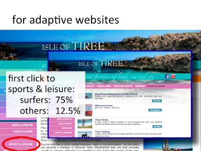
We’ll look at an example of how this can be used to create an adaptive website. This is partly because in this example there is a clear prior probability distribution and the meaning of the posterior is also clear. This will hopefully solidify the concepts of Bayesian techniques before looking at the slightly more complex case of Bayesian statistical inference.
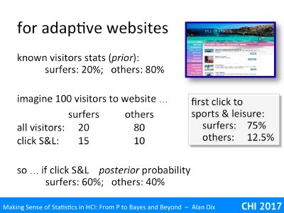
This is the front page of the Isle of Tiree website. There is a menu along the left-hand side; it starts with ‘home’, ‘about Tiree’, ‘accommodation’, and the 12th item is ‘sport & leisure’.
Imagine we have gathered extensive data on use by different groups, perhaps by an experiment or perhaps based on real usage data. We find that for most users the likelihood of clicking ‘sport & leisure’ as the first selection on the site is 12.5%, but for surfers this figure is 75%. Cleary different users access the site in different ways, so perhaps we would like to customise the site in some way for different types of users.
Let’s imagine we also have figures for the overall proportion of visitors to the site who are surfers or non-surfers, let’s say that the figures are 20% surfers, 80% non-surfers. Clearly, as only one in five visitors is a surfer we do not want to make the site too ‘surf-centric’.
However, let’s look at what we know after the user’s first selection.
Consider 100 visitors to the site. On average 20 of these will be surfers and 80 non-surfers. Of the 20 surfers 75%, that is 15 visitors, are likely to click ‘sorts & leisure’ first. Of the 80 non-surfers, 12.5%, that is 10 visitors are likely to click ‘sports & leisure’ first.
So in total of the 100 visitors 25 will click ‘sports & leisure’ first, Of these 15 are surfers and 10 non surfers, that is if the visitor has clicked ‘sports & leisure’ first there is a 60% chance the visitor is a surfer, so it becomes more sensible to adapt the site in various ways for these visitors. For visitors who made different first choices (and hence lower chance of being a surfer), we might present the site differently.
This is precisely the kind of reasoning that is often used by advertisers to target marketing and by shopping sites to help make suggestions.
Note here that the prior distribution is given by solid data as is the likelihood: the premises of Bayesian inference are fully met and thus the results of applying it are mathematically and practically sound.
If you’d like to see how the above reasoning is written mathematically, it goes as follows – using the notation P(A|B) as the conditional probability that A is true given B is true.
Let’s see how the same principle is applied to statistical inference for a user study result.
Let’s assume you are comparing and old system A with your new design system B. You are clearly hoping that your newly designed system is better!
Bayesian inference demands that you make precise your prior belief about the probability of the to outcomes. Let say that you have been quite conservative and decided that:
prior probability A & B are the same: 80%
prior probability B is better: 20%
You now do a small study with four users, all of whom say they prefer system B. Assuming the users are representative and independent, then this is just like tossing coin. For the case where A and B are equally preferred, you’d expect an average 50:50 split in preferences, so the chances of seeing all users prefer B is 1 in 16.
The alternative, B better, is a little more complex as there are usually many ways that something can be more or less better. Bayesian statistics has ways of dealing with this, but for now I’ll just assume we have done this and worked out that the probability of getting all four users to say they prefer B is ¾.
We can now work out a posterior probability based on the same reasoning as we used for the adaptive web site. The result of doing this yields the following posterior:
posterior probability A & B are the same: 25%
posterior probability B is better: 75%
It is three times more likely that your new design actually is better 🙂
This ratio, 3:1 is called the odds ratio and there are rules of thumb for determining whether this is deemed good evidence (rather like the 5% or 1% significance levels in standard hypothesis testing). While a 3:1 odds ratio is in the right direction, it would normally be regarded as a inconclusive, you would not feel able to draw strong recommendations form this data alone.
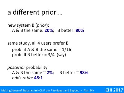
Now let’s imagine a slightly different prior where you are a little more confident in your new design. You think it four times more likely that you have managed to produce a better design than that you have made no difference (you are still modest enough to admit you may have done it badly!). Codified as a prior probability this gives us:
prior probability A & B are the same: 20%
prior probability B is better: 80%
The experimental results is exactly the same, but because the prior beliefs are different the posterior probability distribution is also different:
posterior probability A & B are the same: ~2%
posterior probability B is better: ~98%
The odds ratio is 48:1, which would be considered an overwhelmingly positive result; you would definitely conclude that system B is better.
Here the same study data leads to very different conclusions depending on the prior probability distribution. in other words your prior belief.
On the one hand this is a good thing, it precisely captures the difference between the situations where you toss the coin out of your pocket compared to the showman at the street market.
On the other hand, this also shows how sensitive the conclusions of Bayesian analysis are to your prior expectations. It is very easy to fall prey to confirmation bias, where the results of the analysis merely rubber stamp your initial impressions.
As is evident Bayesian inference can be really powerful in a variety of settings. As a statistical tool however, it is evident that the choice of prior is the most critical issue.
how do you get the prior?
Sometimes you have strong knowledge of the prior probability, perhaps based on previous similar experiments. However, this is more commonly the case for its use in internal algorithms, it is less clear in more typical usability settings such as the comparison between two systems. In these cases you are usually attempting to quantify your expert judgement.
Sometimes the evidence from the experiment or study is s overwhelming that it doesn’t make much difference what prior you choose … but in such cases hypothesis testing would give very high significance levels (low p values!), and confidence intervals very narrow ranges. It is nice when this happens, but if this were always the case we would not need the statistics!
Another option is to be conservative in your prior. The first example we gave was very conservative, giving the new system a low probability of success. More commonly a uniform prior is used, giving everything the same prior probability. This is easy when there a small number of distinct possibilities, you just make them equal, but a little more complex for unbounded value ranges, where often a Cauchy distribution is used … this is bell shaped a bit like the Normal distribution but has fatter edges, like an egg with more white.
In fact, if you use a uniform prior than the results of Bayesian statistics are pretty much identical to traditional statistics, the posterior is effectively the likelihood function, and the odds ratio is closely related to the significance level.
As we saw, if you do not use a uniform prior, or a prior based on well-founded previous research, you have to be very careful to avoid confirmation bias.
handling multiple evidence
Bayesian methods are particularly good at dealing with multiple independent sources of evidence; you simply apply the technique iteratively with the posterior of one study forming the prior to the next. However, you do need to be very careful that the evidence is really independent evidence, or apply corrections if it is not.
Imagine you have applied Bayesian statistics using the task completion times of an experiment to provide evidence that system B is better than system A. You then take the posterior from this study and use it as the prior applying Bayesian statistics to evidence from an error rate study. If these are really two independent studies this is fine, but of this is the task completion times and error rates from the same study then it is likely that if a participant found the task hard on one system they will have both slow times and more errors and vice versa – the evidence is not independent and your final posterior has effectively used some of the same evidence twice!
internecine warfare
Do be aware that there has been an on-going, normally good-natured, debate between statisticians on the relative merits of traditional and Bayesian statistics for at least 40 years. While Bayes Rule, the mathematics that underlies Bayesian methods, is applied across all branches of probability and statistics, Bayesian Statistics, the particular use for statistical inference, has always been less well accepted, the Cinderella of statistics.
However, algorithmic uses of Bayesian methods in machine learning and AI have blossomed over recent years, and are widely accepted and regarded across all communities.
Significance testing helps us to tell the difference between a real effect and random-chance patterns, but it is less helpful in giving us a clear idea of the potential size of an effect, and most importantly putting bounds on how similar things are. Confidence intervals help with both of these, giving some idea of were real values or real differences lie.
So you ran your experiment, you compared user response times to a suite of standard tasks, worked out the statistics and it came out not significant – unproven.
As we’ve seen this does not allow us to conclude there is no difference, it just may be that the difference was too small to see given the level of experimental error. Of course this error may be large, for example if we have few participants and there is a lot of individual difference; so even a large difference may be missed.
How can we tell the difference between not proven and no difference?
In fact it is usually impossible to say definitively ‘no difference’ as it there may always be vanishingly small differences that we cannot detect. However, we can put bounds on inequality.
A confidence interval does precisely this. It uses the same information and mathematics as is used to generate the p values in a significance test, but then uses this to create a lower and upper bound on the true value.
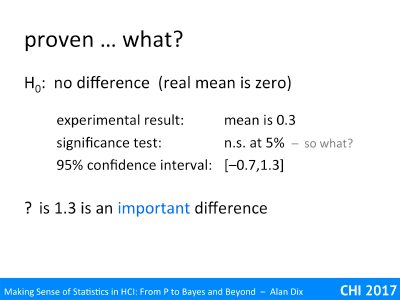
For example, we may have measured the response times in the old and new system, found an average difference of 0.3 seconds, but this did not turn out to be a statistically significant difference.
On its own this simply puts us in the ‘not proven’ territory, simply unknown.
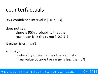
However we can also ask our statistics application to calculate a 95% confidence interval, let’s say this turns out to be [-0.7,1.3] (often, but not always, these are symmetric around the average value).
Informally this gives an idea of the level of uncertainty about the average. Note this suggests it may be as low as -0.7, that is our new system maybe up to 0.7 second slower that the old system, but also may be up to 1.3 seconds faster.
However, like everything in statistics, this is uncertain knowledge.
What the 95% confidence interval actually says that is the true value were outside the range, then the probability of seeing the observed outcome is less than 5%. In other words if our null hypothesis had been “the difference is 2 seconds” or “the difference is 1.4 seconds”, or “the difference is 0.8 seconds the other way”, all of these cases the probability of the outcome would be less than 5%.
By a similar reasoning to the significance testing, this is then taken as evidence that the true value really is in the range.
Of course, 5% is a low degree of evidence, maybe you would prefer a 99% confidence interval, this then means that of the true value were outside the interval, the probability of seeing the observed outcome is less than 1 in 100. This 99% confidence interval will be wider than the 95% one, perhaps [-1,1.6], if you want to be more certain that the value is in a range, the range becomes wider.
Just like with significance testing, the 95% confidence interval of [-0.7,1.3] does not say that there is a 95% probability that the real value is in the range, it either is or it is not.
All it says is that if the real value were to lie outside the range, then the probability of the outcome is less than 5% (or 1% for 99% confidence interval).
Let’s say we have run our experiment as described and it had a mean difference in response time of 0.3 seconds, which was not significant, even at 5%. At this point, we still had no idea of whether this meant no (important) difference or simply a poor experiment. Things are inconclusive.
However, we then worked out the 95% confidence interval to be [-0.7,1.3]. Now we can start to make some stronger statements.
The upper limit of the confidence interval is 1.3 seconds; that is we have a reasonable level of confidence that the real difference is no bigger than this – does it matter, is this an important difference. Imagine this is a 1.3 second difference on a 2 hour task, and that deploying the new system would cost millions, it probably would not be worth it.
Equally, if there were other reasons we want to deploy the system would it matter if it were 0.7 seconds slower?
We had precisely this question with a novel soft keyboard for mobile phones some years ago [HD04]. The keyboard could be overlaid on top of content, but leaving the content visible, so had clear advantages in that respect over a standard soft keyboard that takes up the lower part of the screen. My colleague ran an experiment and found that the new keyboard was slower (by around 10s in a 100s task), and that this difference was statistically significant.
If we had been trying to improve the speed of entry this would have been a real problem for the design, but we had in fact expected it to be a little slower, partly because it was novel and so unfamiliar, and partly because there were other advantages. It was important that the novel keyboard was not massively slower, but a small loss of speed was acceptable.
We calculated the 95% confidence interval for the slowdown at [2,18]. That is we could be fairly confident it was at least 2 seconds slower, but also confident that it was no more than 18 seconds slower.
Note this is different from the previous examples, here we have a significant difference, but using the confidence interval to give us an idea of how big that difference is. In this case, we have good evidence that the slow down was no more than about 20%, which was acceptable.
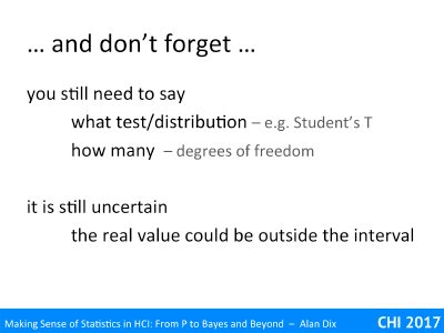
Researchers are often more familiar with significance testing and know that the need to quote the number of participants, the test used, etc.; you can see this in every other report you gave read that uses statistics.
When you quote a confidence level the same applies. If the data is two-outcome true/false data (like the coin toss), then the confidence interval may have been calculated using the Binomial distribution, if it is people’s heights it might use the Normal or Students-t distribution – this needs to be reported so that others can verify the calculations, or maybe reproduce your results.
Finally do remember that, as with all statistics, the confidence interval is still uncertain. It offers good evidence that the real value is within the interval, but it could still be outside.
What you can say
In the video and slides I spend so much time warning you what is not true, I forgot to mention one of the things that you can say with certainty from a confidence interval.
If you run experiments or studies, calculate the 95% confidence interval for each and then work on the assumption that the real value lies in the range, then at least 95% of the time you will be right.
Similarly if you calculate 99% confidence intervals (usually much wider) and work on the assumption that the real value lies in the rage, then at least 99% of the time you will be right.
This is not to say that for any given experiment the probability of the real value lies in the range, it either does or doesn’t. just puts a limit on the probability you are wrong if you make that assumption. These sound almost the same, but the former is about the real value of something that may have no probability associated with it; it is just unknown; the latter is about the fact that you do lots of experiments, each effectively each like the toss of a coin.
So if you assume something is in the 95% confident range, you really can be 95% confident that you are right.
Of course, this is about ALL of the experiments that you or others do . However, often only positive results are published; so it is NOT necessarily true of the whole published literature.
Hypothesis testing is still the most common use of statistics – using various measures to come up with a p < 5% result.
In this video we’ll look at what this 5% (or 1%) actual means, and as important what it does not mean. Perhaps even more critically, is understanding what you can conclude from a non-significant result and in particular remembering that it means ‘not proven’ NOT ‘no effect’!
The language of hypothesis testing can be a little opaque!
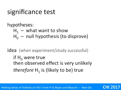
A core term, which you have probably seen, is the idea of the null hypothesis, also written H0, which is usually what you want to disprove. For example, it may be that your new design has made no difference to error rates.
The alternative hypothesis, written H1, is what you typically would like to be true.
The argument form is similar to proof by contradiction in logic or mathematics. In this you assert what you believe to be false as if it were true, reason from that to something that is clearly contradictory, and then use that to say that what you first assumed must be false.
In statistical reasoning of course you don’t know something is false, just that it is unlikely.
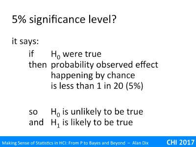
The hypothesis testing reasoning goes like this:
if the null hypothesis H0 were true then the observations (measurements) are very unlikely therefore the null hypothesis H0 is (likely to be) false
and hence the alternative H1 is (likely to be) true
For example, imagine our null hypothesis is that a coin is fair. You toss it 100 times and it ends up a head every time. The probability of this given a fair coin (likelihood) is 1/2100 that is around 1 in a nonillion (1 with 30 zeros!). This seems so unlikely, you begin to wonder about that coin!
Of course, most experiments are not so clear cut as that.
You may have heard of the term significance level, this is the threshold at which you decide to reject the null hypothesis. In the example above, this was 1 in a nonillion, but that is quite extreme.
The smallest level that is normally regarded as reasonable evidence is 5%. This means that if the likelihood of the null hypothesis (probability of the observation given H0) is less than 5% (1 in 20), you reject it and assume the alternative must be true.
Let’s say that our null hypothesis was that your new design is no different to the old one. When you tested with six users all the users preferred the new design.
The reasoning using a 5% significance level as a threshold would go:
if the null hypothesis H0 is true (no difference)
then the probability of the observed effect (6 preference)
happening by chance
is 1/64 which is less than 5%
therefore reject H0 as unlikely to be true
and conclude that the alternative H1 is likely to be true
Yay! your new design is better 🙂
Note that this figure of 5% is fairly arbitrary. What figure is acceptable depends on a lot of factors. In usability, we will usually be using the results of the experiment alongside other evidence, often knowing that we need to make adaptations to generalise beyond the conditions. In physics, if they conclude something is true, it is taken to be incontrovertibly true, so they look for a figure more like 1 in 100,000 or millions.
Note too that if you take 5% as your acceptable significance level, then if your system were no better there would still be a 1 in 20 chance you would conclude it was better – this is called a type I error (more stats-speak!), or (more comprehensibly) a false positive result.
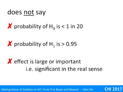
Note also that a 5% significance does NOT say that the probability of the null hypothesis is less than 1 in 20. Think about the coin you are tossing, it is either fair or not fair, or think of the experiment comparing your new design with the old one: your design either is or is not better in terms of error rate for typical users.
Similarly it does not say the probability of the alterative hypothesis (your system is better) is > 0.95. Again it either is or is not.
Nor does it say that the difference is important. Imagine you have lots and lots of participants in an experiment, so many that you are able to distinguish quite small differences. The experiment showed, with a high degree of statistical significance (maybe 0.1%), that users perform faster with your new system than the old one. The difference turns out to be 0.03 seconds over an average time of 73 seconds. The difference is real and reliable, but do you care?
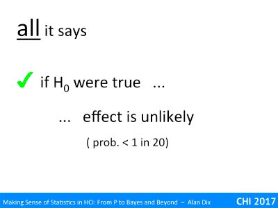
All that a 5% significance level says is that is the null hypothesis H0 were true, then the probability of seeing the observed outcome by chance is 1 in 20.
Similarly for a 1% levels the probability of seeing the observed outcome by chance is 1 in 100, etc.
Perhaps the easiest mistake to make with hypothesis testing is not when the result is significant, but when it isn’t.
Say you have run your experiment comparing the old system with the new design and there is no statistically significant difference between the two. Does that mean there is not difference?
This is a possible explanation, but it also may simply mean your experiment was not good enough to detect the difference.
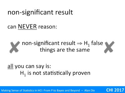
Although you do reason that significant result means the H0 is false and H1 (the alternative) is likely to be true, you cannot do the opposite.
You can NEVER (simply) reason: non-significant result means H0 is true / H1 is false.
For example, imagine we have tossed 4 coins and all came up heads. If the coin is fair the probability of this happening is 1 in 16, this is not <5%, so even with the least strict level, this is not statistically significant. However, this was the most extreme result that was possible given the experiment, tossing 4 coins could never give you enough information to reject the null hypothesis of a fair coin!
Scottish law courts can return three verdicts: guilty, not guilty or not proven. Guilty means the judge or jury feels there is enough evidence to conclude reasonably that the accused did the crime (but of course still could be wrong) and not guilty means they are reasonably certain the accused did not commit the crime. The ‘not proven’ verdict means that the judge or jury simply does not feel they have sufficient evidence to say one way or the other. This is often the verdict when it is a matter of the victim’s word versus that of the accused, as is frequently happens in rape cases.
Scotland is unusual in having the three classes of verdict and there is some debate as to whether to remove the ‘not proven’ verdict as in practice both ‘not proven’ and ‘not guilty’ means the accused is acquitted. However, it highlights that in other jurisdictions ‘not guilty’ includes both: it does not mean the court is necessarily convinced that the accused is innocent, merely that the prosecution has not provided sufficient evidence to prove they are guilty. In general a court would prefer the guilty walk free than the innocent are incarcerated, so the barrier to declaring ‘guilty’ is high (‘beyond all reasonable doubt’ … not p<5%!), so amongst the ‘not guilty’ will be many who committed a crime as well as many who did not.
In statistics ‘not significant’ is just the same – not proven.
In summary, all a test of statistical significance means is that if the null hypothesis (often no difference) is true, then the probability of seeing the measured results is low (e.g. <5%, or <1%). This is then used as evidence against the null hypothesis. It is good to return to this occasionally, but for most purposes an informal understanding is that statistical significance is evidence for the alterative hypothesis (often what you are trying to show), but maybe wrong – and the smaller the % or probability the more reliable the result. However, all that non-significance means is not proven.
You use statistics when there is something in the world you don’t’ know, and want to get a level of quantified understanding of it based on some form of the measurement or sample.
One key mathematical element of this shared by all techniques is the idea of conditional probability and likelihood; that is the probability of a specific measurement occurring assuming you know everything pertinent about the real world. Of course the whole point is that you don’t know what is true of the real world, but do know about the measurement, so you need to do back-to-front counterfactual reasoning, to go back from measurement to the world!
Future videos will discuss three major kinds of statistical analysis methods:
Hypothesis testing (the dreaded p!) – robust but confusing
Confidence intervals – powerful but underused
Bayesian stats – mathematically clean but fragile
The first two use essentially the same theoretical approach, and the difference is more about the way you present results. Bayesian statistics takes a fundamentally different approach, with its own strengths and weaknesses.
First of all let’s recall the ‘job of statistics‘, which is an attempt to understand the fundamental properties of the real world based on measurements and samples. For example, you may have taken a dozen people (the sample), asked them to perform a task on a piece of software and a new version of the software. You have measured response times, satisfaction, error rate, etc., (the measurement) and want to know whether your new software will out perform the original software for the whole user group (the real world).
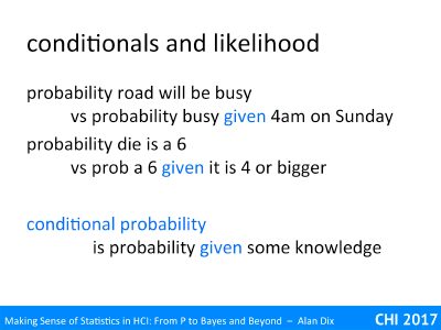
We are dealing with data with a lot of randomness and so need to deal with probabilities, but in particular what is known as conditional probability.
Imagine the main street of a local city. What is the probability that it is busy?
Now imagine that you are standing in the same street but it is 4am on a Sunday morning: what is the probability it is busy given this?
Although the overall probability of it being busy (at a random time of day) is high, the probability that it is busy given it is 4am on a Sunday is lower.
Similarly think of a throwing single die. What is the probability it is a six? 1 in 6.
However, if I peek and tell you it is at least 4. What now is the probability it is a six? The probability it is a six given it is four or greater is 1 in 3.
When we have more information, then we change our assessment of the probability of events accordingly. This calculation of probability given some information is what mathematicians call conditional probability.
Returning to the job of statistics, we are interested in the relationship between measurements of the real world and what is true of the real world. Although we may not know what is true of the world (what is the actual error rate of our new software going to be), we can often work out the probability of measurements given (the unknown) state of the world.
For example, if the probability of a user making a particular error is 1 in 10, then the probability that exactly 3 make the error out of a sample of 5 is 7.29% (calculated from the Binomial distribution).
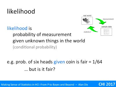
This conditional probability of a measurement given the state of the world (or typically some specific parameters of the world) is what statisticians call likelihood.
As another example the probability that six tosses of a coin will come out heads given the coin is fair is 1/64, or in other words the likelihood that it is fair is 1/64. If instead the coin were biased 2/3 heads 1/3 tails, the probability of 6 heads given this, likelihood fo the coin having this bias, is 64/729 ~ 1/ 11.
Note this likelihood is NOT the probability that the coin is fair or biased, we may have good reason to believe that most coins are fair. However, it does constitute evidence. The core difference between different kinds of statistics is the way this evidence is used.
Effectively statistics tries to turn this round, to take the likelihood, the probability of the measurement given the unknown state of the world, and reverse this, use the fact that the measurement has occurred to tell us something about the world.
Going back again to the job of statistics, the measurements we have of the world are prone to all sorts of random effects. The likelihood models the impact of these random effects as probabilities. The different types of statistics then use this to produce conclusions about the real world.
However, crucially these are always uncertain conclusions. Although we can improve our ability to see through the fog of randomness, there is always the possibility that by shear chance things appear to suggest one conclusion even though it is not true.
We will look at three types of statistics.
Hypothesis testing is what you are most likely to have seen – the dreaded p! It was originally introduced as a form of ‘quick hack’, but has come to be the most widely used tool. Although it can be misused, deliberately or accidentally, in many ways, it is time-tested, robust and quite conservative. The downside is that understanding what it really says (not p<5% means true!) can be slightly complex.
Confidence intervals use the same underlying mathematical methods as hypothesis testing, but instead of taking about whether there is evidence for or against a single value, or proposition, confidence intervals give a range of values. This is really powerful in giving a sense of the level of uncertainty around an estimate or prediction, but are woefully underused.
Bayesian statistics use the same underlying likelihood (although not called that!) but combine this with numerical estimates of the probability of the world. It is mathematically very clean, but can be fragile. One needs to be particularly careful to avoid conformation bias and when dealing with multiple sources of non-independent evidence. In addition, because the results are expressed as probabilities, this may give an impression of objectivity, but in most cases it is really about modifying one’s assessment of belief.
We will look at each of these in more detail in coming videos.
To some extent these techniques have been pretty much the same for the past 50 years, however computation has gradually made differences. Crucially, early statistics needed to relatively easy to compute by hand, whereas computer-based statistical analyses can use more complex methods. This has allowed more complex models based on theoretical distributions, and also simulation methods that use models where there is no ‘nice’ mathematical solution.
In this part we will look at the major kinds of statistical analysis methods:
Hypothesis testing (the dreaded p!) – robust but confusing
Confidence intervals – powerful but underused
Bayesian stats – mathematically clean but fragile
None of these is a magic bullet; all need care and a level of statistical understanding to apply.
We will discuss how these are related including the relationship between ‘likelihood’ in hypothesis testing and conditional probability as used in Bayesian analysis. There are common issues including the need to clearly report numbers and tests/distributions used. avoiding cherry picking, dealing with outliers, non-independent effects and correlated features. However, there are also specific issues for each method.
Classic statistical methods used in hypothesis testing and confidence intervals depend on ideas of ‘worse’ for measures, which are sometimes obvious, sometimes need thought (one vs. two tailed test), and sometimes outright confusing. In addition, care is needed in hypothesis testing to avoid classic fails such as treating non-significant as no-effect and inflated effect sizes.
In Bayesian statistics different problems arise including the need to be able to decide in a robust and defensible manner what are the expected prior probabilities of different hypothesis before an experiment; the closeness of replication; and the danger of common causes leading to inflated probability estimates due to a single initial fluke event or optimistic prior.
Crucially, while all methods have problems that need to be avoided, not using statistics at all can be far worse.
Thing to come …
probing the unknown
conditional probability and likelihood
statistics as counter-factual reasoning
types of statistics
hypothesis testing (the dreaded p!) – robust but confusing
confidence intervals – powerful but underused
Bayesian stats – mathematically clean .. but fragile – issues of independence
 Now here is a small exercise to get a feeling for that p < 5% figure … are your coins really fair?