These techniques rely on using the internal representation of the black-box algorithm as an opaque feature vector from which other forms of white and black-box algorithms can be applied in order to obtain humanly meaningful results or create other learned representations.
There are two forms of internal representation at play here:
- (i) The parameters, such as NN weights that are learnt during training and are then usually static during use.
- (ii) The internal activations of nodes or other forms of intermediate calculations that vary for each input.
The exact form of these will be different for different kinds of algorithm, but as a generic term we’ll use the term parameters for the former and activation for the latter.
For temporal networks (ii) gets a little more complex as the same input might generate a different internal activation. However, the majority of such algorithms have some form of internal representation of state where the rest of the algorithm can be seen as calculating:
state’, output = f ( parameters, state, input)
So, if we regard the state–input pair as the input, we can effectively, without loss of generality, consider only simple non-temporal input–output algorithms.
Again for the case of simplicity, we’ll refer to the site of atomic calculations within an algorithm as nodes, thinking of NNs as central example, but this might also be, for example, branches in a decision tree.
Also the internal representation may often be layered (esp. DL), with lower layers closer to the input, one or more intermediate layers and a high layer that generates the output.
GB0. Sensitivity analysis.
Several techniques can benefit from some form of sensitivity analysis to allow pruning/simplification or add weights/uncertainty factors for other algorithms.
There are at least three ways this can be done.
(GB0a) Focus on the parameters (e.g. NN weights) – perturb these and see if this affects the overall goodness of fit of the representation.
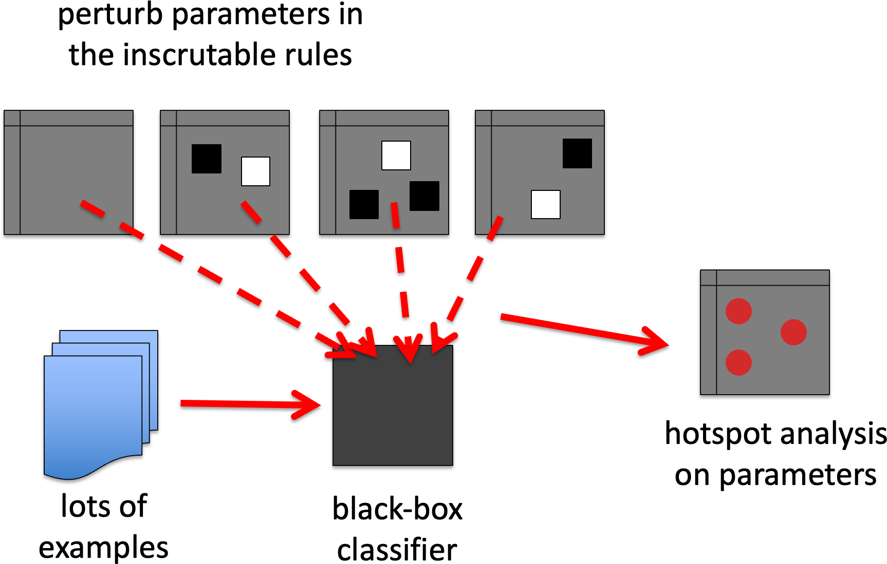
GB0a. sensitivity analysis – weights
(GB0b) Focus on the activation – perturb the outputs of individual nodes for specific inputs and see whether this affects the overall output.
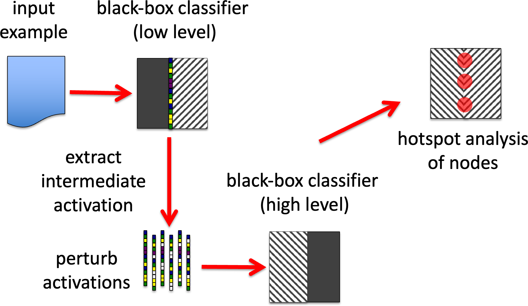
GB0b. sensitivity analysis – activation
(GB0c) Algorithmically – use some formula to derive this, for example, back- propagation in a NN.
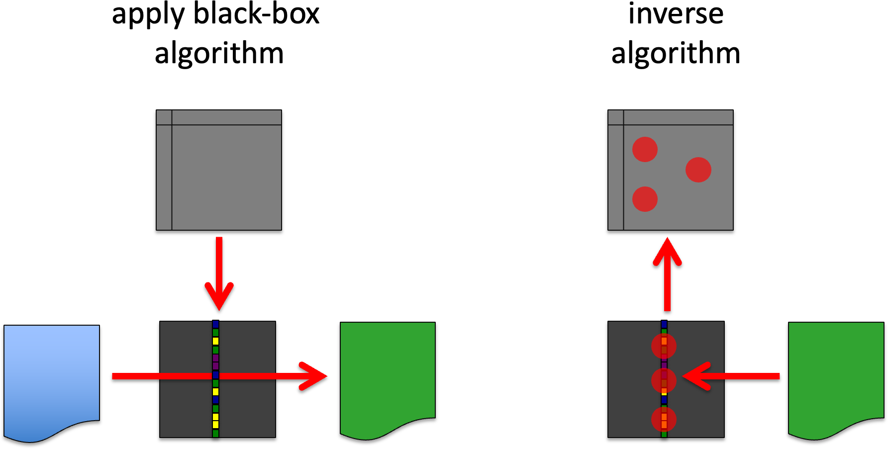
GB0c. sensitivity analysis – algorithmic
GB1. High level model generation.
Intermediate activation, possibly paired with the raw input, is used as the feature vector for some form of white-box learning algorithm that generates the output from these. That is one is seeking to replace the top level(s) of the representation with one that is easier to understand.
Effectively we are seeing the inscrutable algorithm as operating in two parts:
activationint = flow ( input )
output = fhigh (activationint )
We then are seeking to recreate fhigh using a more comprehensible learning algorithm.
By comparison with a human exert, the aim is to have a level of explanatory model that is like a doctor saying, “this skin patch worries me because it is dark and irregular”. The meanings of ‘dark and ‘irregular’ may well be ones that one can only make sense of by looking at examples, but the high level decision making is explicit.
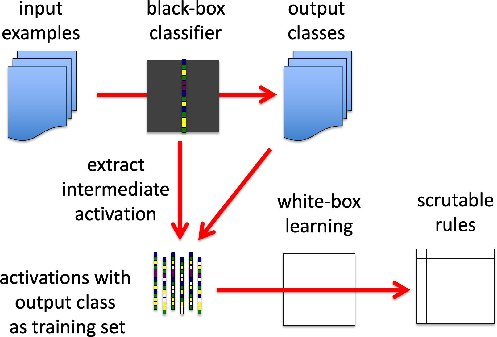
GB1. high level model generation
GB2. Clustering and comprehension of low level.
Here we focus on the mapping from input to intermediate activation.
We effectively treat the intermediate activation (or a subset of it) as a feature vector (rather than the input) and seek to find clusters or other ways to organise the input space (e.g. multi-dimensional scaling, self- organising nets). This may involve initially reducing the example set to a similarity matrix where the cosine or other distance metric is used on the intermediate activations of each pair of examples.
Here we are trying to find ways to understand flow: not primarily intending to replace it (although sometimes this may be possible), but to help create more comprehensible representations of the way it segments the input space.
With the medical example, this would be like creating sets of examples of different features such as ‘irregular’ or ‘dark. The centre/boundary exploration of BB3 may be useful here, but focused on the implicit classes revealed in the intermediate activation rather than the final output.
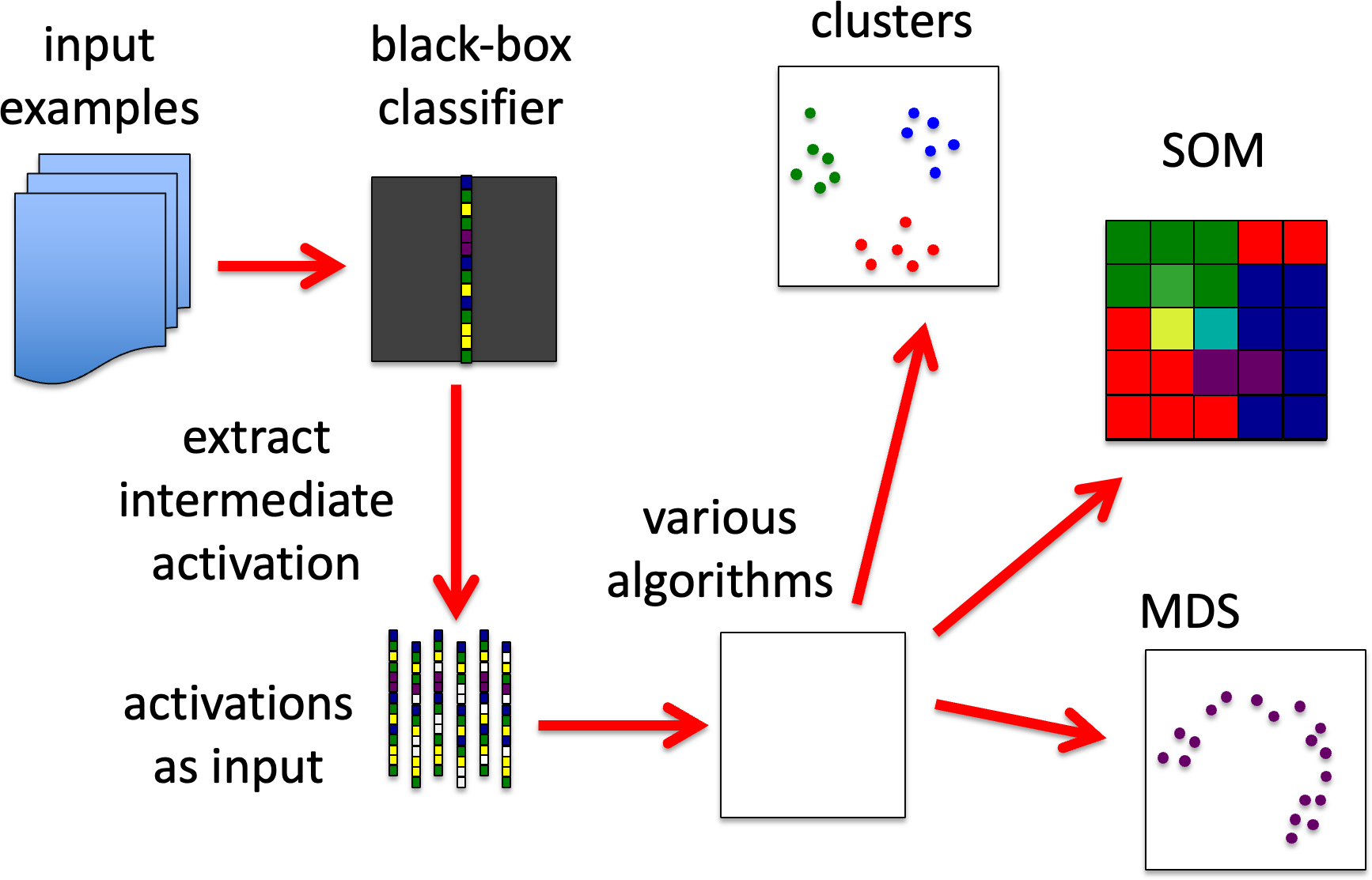
GB2. Clustering and comprehension of low level
GB3. Triad distinctions.
This consists of taking triples of inputs A, B, C, where A and B are members of one class and C of another (or maybe self-organising versions without this constraint). The activations for A, B and C are examined to find main areas where A is similar to B, but different from C.
This is effectively an automated variant of the technique initially used in repertory grid interviews and then been adopted for human expertise elicitation.
This can be used as a form of weighting/hotspot detection – so can be used like GB0 to help tune GB1 or GB2, or may be used to help in key feature detection, as in BB3. However, unlike BB3, this would be most likely used for actual known-value training set rather than generated examples.
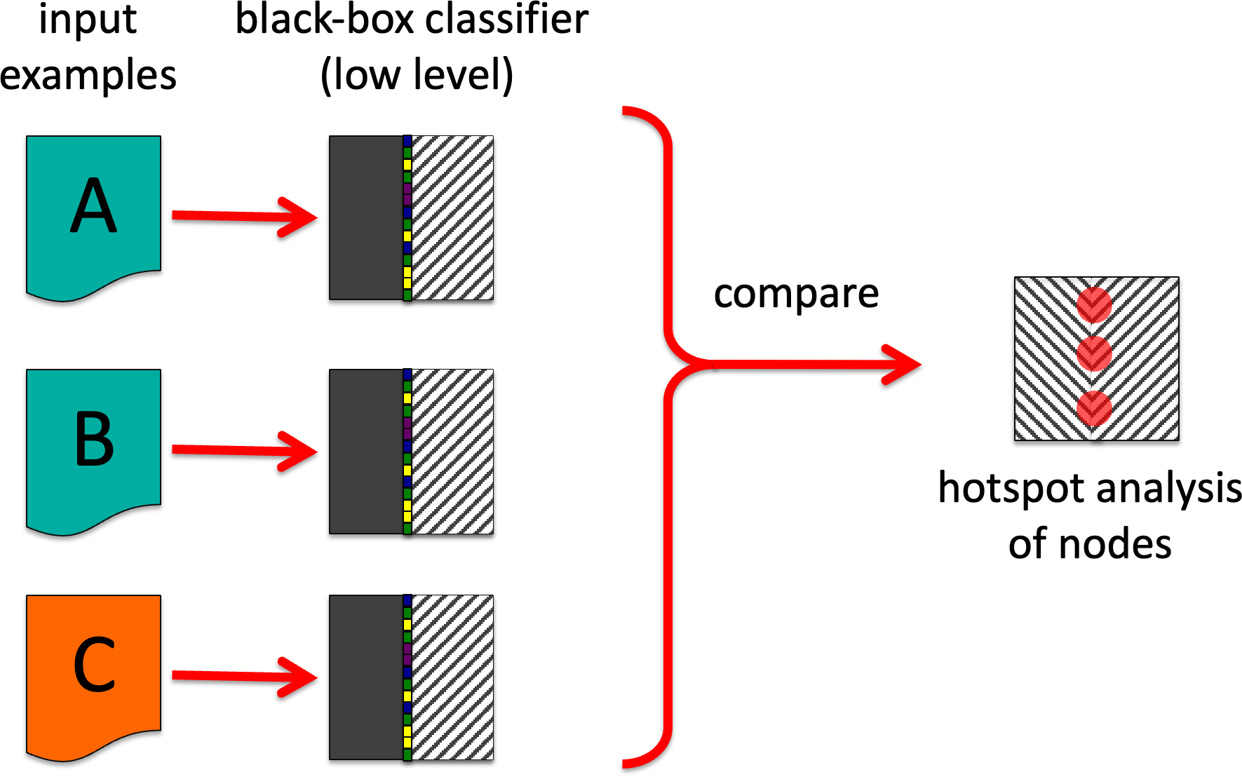
GB3. Triad distinctions
GB4. Apply generatively.
Use the workings of the algorithm to generate inputs or intermediate activations that would give rise to a given final output feature or intermediate activation. That is effectively invert f, flow; or fhigh.
You probably cannot fully invert these, but may be able to algorithmically help for the search of central or boundary cases BB3. For example, in a NN, backprop is effectively computing a point partial differential of output wrt node weights (parameters), which is then used to hill-climb the weights (for NN effectively a pseudo-stochastic hill- climb). However, the backprop procedure also gives (as a freebie!) the partial differential wrt inputs and activation; it thus enables hill- climbing (simulated annealing, etc.) on these as well.
The outputs of this may be used to drive other algorithms or as part of visualisation – the precise ‘rules’ for a effectively fuzzy distinction (e.g. ‘irregular’) may be hard to grasp, but examples may make it obvious.
In general apply your favourite method to some portion of the internal activation as a feature vector 🙂
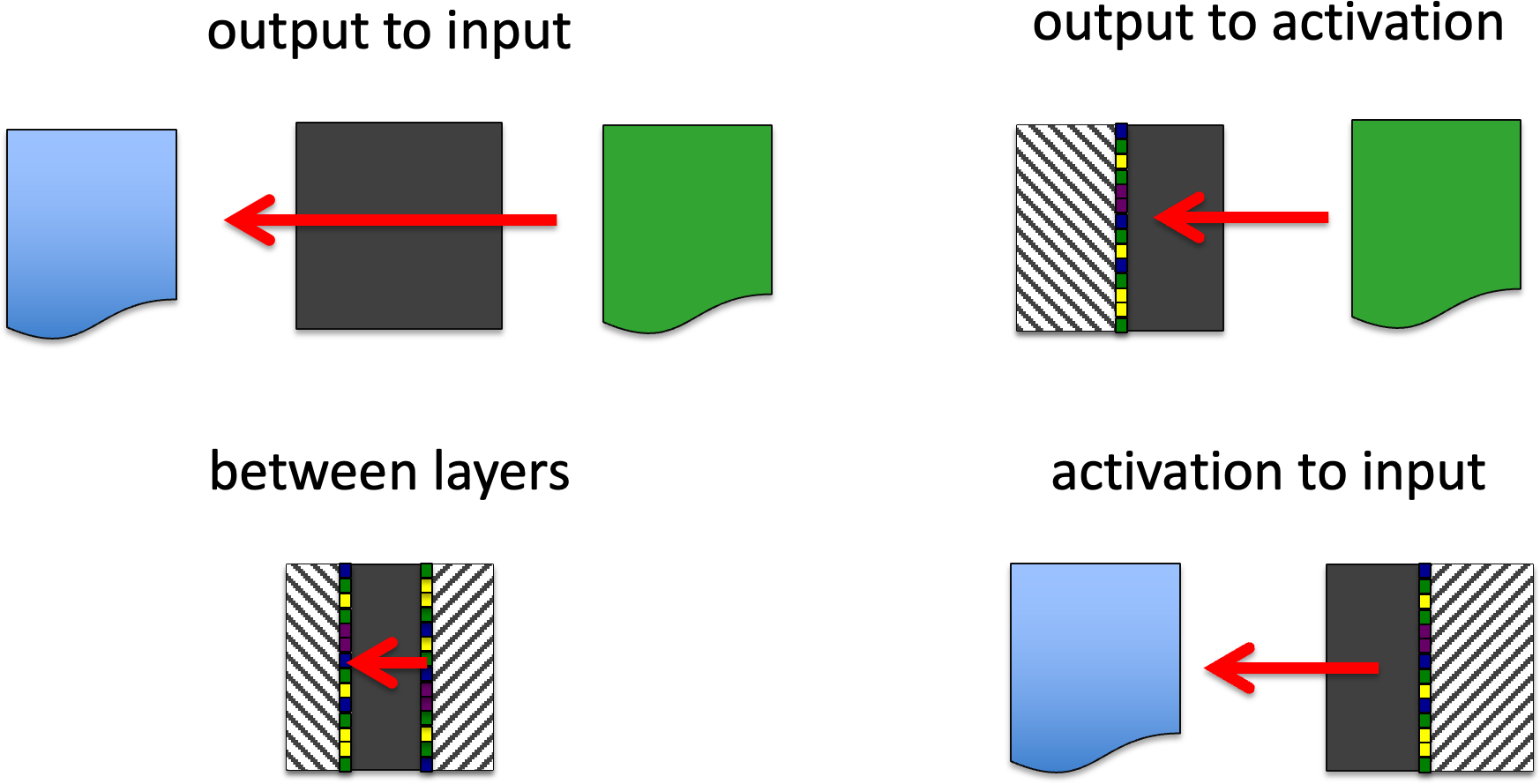
GB4. apply generatively
