See the full draft paper (Adobe PDF).

Full reference:

Alan Dix (1999).
Three DSP Tips. Technical Report, Staffordshire University.
http://www.hcibook.com/alan/papers/DSP99/

Abstract

Some years ago the author was involved in a project which required the detection and location of signals where the signal-to-noise ratio was between 0.001 and 0.0001 - that is, the signal was over 1000 times weaker than the background noise. This report describes three 'tricks' used to solve this problem:

1. hand massaging of digital filters to remove DC bias;
2. using time dependent filters to shift target frequencies to zero Hz and so allow undersampling and more complex processing at slower clock speeds;
3. non-linear correlation filtering for stereo signals to extract common, but possibly phase shifted, signals from multiple detectors with independent noise at each source.

keywords: digital signal processing, signal-to-noise ratio, covariance, band-pass filter, Fourier analysis, stereo, real-time programming

Introduction

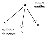
Some years ago, the author was involved in a project to detect and track an emitter of fixed frequency signal using several independent detectors.  With no background noise it would have simply involved a form of triangulation between the detectors to determine the target position.  The reality was more complex than that, with enormous (slowly changing) DC bias at each detector and noise generated by motors and other equipment.  The signals being detected were electromagnetic, but the techniques could be used for acoustic or other types of signal.

The problem

A single emitter is producing signals at a known frequency w0 with some slow time-dependent amplitude change as the emitter moves relative to the detectors.  There is a large time-varying DC bias that is partly common to the detectors and partly independent.  Large here means a noise-to-signal ration of 1000 to 10 000 to 1.  That is our noise swamps the signal several thousand fold!  There were also multiple external sources of other frequency noise.

Figure 1.    emitter and detectors

The circumstances are quite specific, but are not that different from, for example, locating a mobile phone from its signal strength at several base locations.  In this case, there may well be large scale, slowly varying, electromagnetic fields caused by atmospheric conditions.  These could be many times stronger than the phone signals and pose a similar problem.

Similarly, for stereo acoustic detection, there will be slow pressure changes in the air caused by winds and other atmospheric effects, but also other sources of noise.

The simplifying feature of the problem dealt with here is the known fixed target frequency, but the some of the techniques can be applied to unknown frequencies, where the calculations are effectively reproduced in parallel for a set of Fourier frequencies.

Critical factors

Let's look at the implications of the various factors.

fixed frequency signal

Although this frequency is known it is not possible to know that the clocks at the emitter and detectors are 100% accurate with respect to one another.  That is a nominal 100 Hz could easily be 101 Hz or 99 Hz.  Thus the fixed frequency can help us, but an extremely narrow band pass filter could lose the signal.  Although the signal was known, it varied from emitter to emitter and so the hardware analogue filters had to have a broad enough band-pass to cope with a range of target frequencies – only at the digital stage was the exact frequency known.

amplitude modulation signal

The amplitude modulation effectively introduces a slow time-dependant phase shift to the signal.  This again means that a very narrow band pass filter would destroy the signal.

time varying DC bias

If the DC bias were fixed it could be removed by the simplest of analogue or digital filters.  However, as the bias changes slowly with time meaning it 'leaks' into other frequency ranges, including our target frequency.  Recalling the large noise-to-signal ratio, this is a significant effect.

large noise-to-signal ratio

With 14 bit AD capture and a noise to signal ratio of up to 10 000 to 1, it is clear that the real signal will only be able to affect the bottom few bits of the captured signal.  pre-filtering with analogue band-pass filters reduced the noise somewhat, but could not, for various practical reasons, achieve massive reductions.

independent other noise sources

The non-DC external sources were far less strong than the DC bias (but still significant).  However, it was possible (and in some cases likely) that they would produce noise within the target frequency range.  Thus digital and analogue band-pass filtering would tend to leave some of these in as well as the DC leakage.  The only redeeming feature is that this kind of noise was, in the particular problem situation, largely independent at each detector.  In our case this was because the external sources of noise tended to be closer to one detector or another, but it would also be the case for noise generated internally at the sensors.

Solution architecture

In order to deal with the above problem a five stage solution was used:

(i) analogue band-pass filter  (broad)
(ii) digital band-pass filter  (tuned to target frequency)
(iii) single point time-dependent Fourier filter
(iv) correlation filtering
(v) triangulation (using the recovered signal)

The first stage is standard and the last stage particular to the application domain and commercially sensitive.  The middle three stages are discussed in this report.  These techniques could be used together or independently for different kinds of problem.

In the system we developed stage (i) was performed in hardware.  The analogue signal was captured using 14 bit A-D converters.  Stages (ii) and (iii) were performed within an interrupt handler which had to be guaranteed to finish within the sampling period t.  Any complex processing had to be avoided.  The interrupt routine therefore passed values for each sensor through to a main program loop in which subsequent processing of stages (iv) and (v) was performed.  This main loop operated at a slower rate  than the interrupt routine due to undersampling between stages (iii) and (iv).

Technique 1  –  hand massaging digital filters

Problem: automatically generated integer digital filters
Solution: modify integer coefficients to improve specific DC attenuation

The digital filters in stage (ii) were generated using a computer package.  Given parameters, such as a band-pass window, tolerance at the edges of the window, choice of filter type (including several types of both IIR and FIR), the package found an optimal filter and could then output this in a number of forms including calculations using integer coefficients.  The latter was chosen for the target application because the integer calculations on the chosen DSP chip were far faster than its floating point calculations.
The generated filter was a multi-stage IIR type where stage 0 was the input signal and each stage(x[i]) was calculated from the previous stage (x[i-1]) using a calculation of the form:

x[i]t   =  (a x[i]t-1  +  b[i]0 x[i-1]t  +  b[i]1 x[i-1]t-1  +  b[i]2 x[i-1]t-2)  / scale[i]

The rescaling at the end was included by the package to obtain a unit gain in the filter overall.  However, because the signal was only being captured in the lowest bits of the A-D it was desirable to add gain wherever possible and the scale factor was reduced accordingly.  (N.B. the scale factor was, of course, chosen to be a power of two and implemented as a shift!)  However too much gain would lead to integer overflow.  The faster the initial stages could reduce the noise level, the higher the gain could be in these stages increasing the sensitivity of the device.

A close examination of the coefficient triples b0, b1, b2 were typically values like:

643, -1285, 643        or         1013,-2027,1013

From the mathematics of the chosen filters and examination, it was clear these were intended to be of an elliptic form:  b, -2b, b, but that rounding to integers gave the slight discrepancies.  The pure filter would of course destroy a DC bias completely, but the rounded one merely attenuated it.  A simple hand editing of these coefficients to values such as:

643, -1286, 643        or         1013,-2026,1013

Killed the troublesome DC bias and led to an instant 10 fold increase in sensitivity of the filter!

Although the precise circumstances were particular to our problem, the general advice is to look carefully at such automatically generated figures.  A small tweak can lead to massive improvements.

Technique 2  –  time dependent Fourier filter

Problem: need more filtering then CPU time available

Solution: use time-dependent filter and under-sampling

After the above digital filtering there was still a significant amount of noise (recall that the original noise-to-signal ratio was 10 000!).  Furthermore some of this noise was within the target signal band.  More sophisticated filtering was obviously required.  However, CPU resources were near their limits.  The problem was, how to do more filtering with only a small amount of free time resources.  Processing at the full signal rate was impossible.

The solution adopted was, once every cycle of the target frequency, to do a one point Fourier transform of the signal and use the output of this as a new, signal with a slower rate.

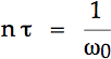
Given the target frequency w0, assume that its period is exactly n of the underlying clock ticks.  That is if the sampling period is t:

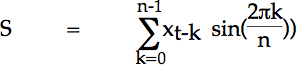
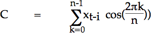
Then every n ticks, two values S and C are calculated from the filtered signal xt.

As is evident, this constitutes a single value from the full Fourier transform over the n samples of the signal.

The resulting values S and C, sampled once every n ticks of the underlying sample rate, become the signal for future processing.

The process of generating S and C can be seen as a form of band pass filter in itself.  More important the combined effect of multiplying by a sine/cosine filter and undersampling at the cosine frequency has the effect of shifting the frequency of the signal.

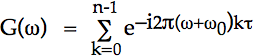
This can most easily be seen using a complex Fourier transform.  Imagine we are calculating the output at every time step, not just once per period.  Consider the component of the input signal, X(w)ei2pw t, at  frequency w.  We imagine we are multiplying the signal by time dependent filter with period w0.  Because we are undersampling this has exactly the same effect as our sine/cosine convolution.  The filtered value of X(w) is:

The last term of this:

Is the gain at frequency w.

The first part is the time varying signal.  But note it is at w+w0 rather than w.  In fact, a real signal at frequency w will have complex components at frequency ± w, so the real signal will end up with components at (w+w0) and (w-w0).

The result of all this is that part of the target signal at w0 is transformed to zero Hz![1]  This means our original fast varying signal is now slowly varying and we have far more time to do complicated filtering.

Technique 3  –  correlation filters

Problem: multiple data streams with correlated signal and uncorrelated noise

Solution: build signal correlation at specific frequency

We now have a slowly varying signal operating near zero Hz.  One solution would be to simply average the signal over a long time period.  Alternatively we could have performed some more band pass filtering at 0 Hz (averaging is effectively a simple band pass filter for 0 Hz anyway!).  However, we have 3 problems:

(i) aliased noise – There is some noise at the target frequency.  One of the potential target frequencies happened to be 50 Hz, which of course is the normal AC operating frequency in the UK, so there would be much interference from AC motors etc.

(ii) target accuracy – There may be a small difference between clock used to drive the signal emitter and the clock at the detectors, meaning the signal could end up just outside a very narrow band pass filter.

(ii) signal modulation – The signal is slowly changing in amplitude and phase due to movement of the detectors relative to the emitter.  This means that the signal is effectively spread over a slightly wider bandwidth and would again be destroyed by a very narrow band pass filter, even if both emitter and detectors have perfect frequency match.[2]

With a single detector we would probably have to content with the level of signal we had.  There would be no way of distinguishing the emitter's signal from other noise at the target frequency.  However, we have one advantage – multiple detectors.  In our application, the signal was common to all detectors (although there would be amplitude and phase differences) and the main noise sources were different for each detector.

If we treat the C and S values at each detector, d,  as a complex signal sd(t), we can model the signals as:

sd(t)    =     kde(t)  +  nd(t)

where e(t) is the emitter signal, kd is the (complex number representing) the phase and amplitude  shift of e(t) at detector d, and nd(t) is the noise at detector d.

Note that kd is precisely the value we would like to recover.  The difference in amplitude is precisely the information required to perform triangulation..  In our case, the phase difference was largely due to sampling strategy, but with acoustic or seismic signals the phase difference could also be useful information.

In fact, the k values themselves vary slowly over time (problem iii), but (happily) it turned out that the timescale for (iii) was slow enough to be ignored in this stage of processing.  This effectively puts a time limit on the whole process – results need to be delivered at a pace similar to the rate of change of the measured phenomena!

The noise from each detector is assumed to be independent.  This means that the correlation between two detectors' noise is zero:(averaged over a sufficiently long period):

N.B.  E is the statistical 'expected' value and this means that over a sufficiently long time the average will be approximately zero

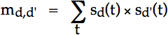
This gives us the means to perform a 'correlation' filter.  For each pair of complex signals we compute a time averaged product.  This builds a covariance matrix:

Expanding this we get:

The latter three terms average to zero over a long period meaning that the calculated covariance matrix becomes an accurate estimate of the matrix obtained by multiplying the k values together (outer product of the 'k vector'):

The scaling factor  is simply the overall signal strength, which was measured independently using simpler algorithms!  The matrix values allow the comparative values of the k's to be recovered.

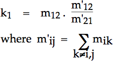
The only complication in recovering the k values is that the matrix values corresponding to signals at the same detector had to be ignored.  We actually had x,y,z channels at each detector, which of course would be subject to potentially correlated noise.  These values were discarded, leaving a partial matrix (Fig. 2).  Happily, the out product matrix is so redundant it is still easily possible to recover the k values.  Either using a least squares solution, or a simpler closed solution such as:

Figure 2.    partial covariance matrix

Summary

The three 'tips' presented here were developed as part of a solution to a specific problem.  They each address different aspects of the problem and so may be useful in other circumstances.

1. hand tweaking of digital filters  –  A good idea for any automatically generated integer coefficient filter.  You can then use automatic tools or analytic calculations to test which of the 'close' digital versions is best.

2. frequency shifting using Fourier filter and undersampling  –  This can be used in any application where pre-filtering can reduce the bandwidth to avoid aliasing.

3. correlation filtering  –  This can be used wherever there is stereo or other multi-detector input .

To the best of my knowledge (3) is a completely original method, (2) is a different way of looking at undersampling and (1) is sheer computer hackery!

However, as an academic, DSP is not my specialist area – I am simply a practitioner, so I would welcome any information on similar techniques used elsewhere.

The take away message is not just that there are three useful techniques, but that for a specific problem one cannot simply take pre-packaged techniques of the shelf.  Instead, one needs to look at the particular conditions of the situation, both its problems and its opportunities.  An appropriate solution will often involve tweaking existing methods or developing tailored ones for the problem at hand.

Bibliography

I've read many books on aspects of Fourier analysis, but own few.  The best introductory ones usually have titles like "Mathematics for Engineers".  The book I use as a basic reference is:

• O. L. R. Jacobs (1974). Introduction to Control Theory.  Oxford University Press.

For coding examples of Fourier transforms, digital filters and much else, the only place is:

• W. H. Press, B. P. Flannery, S. A. Teukolsky and W. T. Vetterling (1988). Numerical recipies in C  Cambridge University Press.

Finally for information about physical tranducers:

• C. Loughlin (1993). Sensors for Industrial Inspection.  Kluwer Academic Publishers.

Appendix  –  some more tips for real time programming

If you are implementing DSP algorithms you will probably be trying to write fast code, often with real-time constraints, such as catching interrupts.  So, as well as the DSP tips there are a few real computer hacker ones as well, for tight real-time systems programming.

• know your platform –– rules change so check them out!

• you should know this, but ... where possible use shifts instead of multiply and divide

• where possible use integers instead of floats

• favour integer sizes that match the platform – not necessarily the smallest.  Memory access and arithmetic operations will usually be most efficient at the machine's natural precision.

• inlining functions does not always make code faster  –  I don't know why, I guess compilers do worse register allocation!

• loop unrolling does not always make code faster  –  For the same reason as above, also if the machine has an instruction cache a small loop may fit entirely in the cache whereas the unrolled loop will demand constant memory accesses.

• write the slowest code possible not the fastest  – Wait do I really mean that?  Well, not quite ...

• write code with predictable timings  –  In real time processes don't have lots of clever conditions that make the code faster most of the time, but sometimes leave a slower alternative.  When you test the code you will hit the fast ones and only when it is deployed will the slow case occur, possibly forcing missed interrupts, lost data etc. etc.  If the code always runs the same speed testing gives you accurate timings – if it runs fast enough during testing, it won't fail in the field!

Footnotes