 |
More substantial tossing experiments with virtual coins. |
Documentation
This application is very similar to the Two Horse Races demo, except no race track!
This does not do a two-horse race, but instead will toss a given number of coins, and then repeat this. You don’t have to press the toss button for each coin toss, just once and it does as many as you ask.
Instead of the virtual race area, there is just an area to put the number or coins you want it to toss, and then the number of rows of coins you want it to produce.
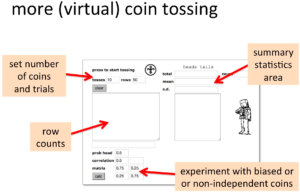
More (virtual) coin tossing – main screen areas
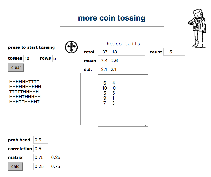
Let’s look in more detail (below). At the top right are text areas to enter the number of coins to toss (here 10 coins at a time) and the number of rows of coins (here set to 50 rows). You press the coin to start, just as in the two-horse race, except now it will toss the coin 10 times and the Hs and Ts will appear in the tally box below. Once it has tossed the first 10 it will toss 10 more, and then 10 more until it has 50 rows of coins — 500 in total … all just for one press.
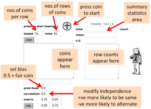
More (virtual) coin tossing — details
The area for setting bias and correlation is the same as in the two-horse race, as is the statistics area.
Let’s look at a few examples runs.
Fair coins
The first run (below) shows a set of tosses where the coin was set to be fair (prob head=0.5) with completely independent tosses (correlation=0) — that is just like a real coin (only faster).
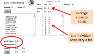
Fair coin (independent tosses)
You can see the first 9 rows and first 9 row counts in the left and right text areas. Note how the individual rows vary quite a lot, as we have seen in the physical coin tossing experiments. However, the average (over 50 sets of 10 coin tosses) is quite close to 50:50. Note also the standard deviation
The standard deviation is 1.8, but note this is the standard deviation of the sample. Because this is a completely random coin toss, with well understood probabilistic properties, it is possible to calculate the `real’ standard deviation — this is the value you would expect to see if you repeated this thousands and thousands of times. This value is the square root of 2.5, which is just under 1.6. This measured standard deviation is an estimate of the `real’ value, and hence not the `real’ value, just like the measured proportion of heads has tuned out at 0.49, not exactly a half. This estimate of the standard deviation itself varies a lot … indeed estimates of variation are often very variable themselves!
Biased coins
The next run (below) shows another set of tosses, this time with the probability of a head set to 0,25. That is a (virtual!) coin that falls heads about a quarter of the time. So a bit like having a four sided spinner with heads on one side and tails on the other three.
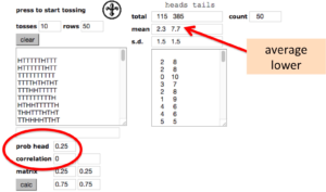
Biased coin (independent tosses)
The correlation has been set to zero still so that the tosses are independent.
You can see how the proportion of heads is now smaller, on average 2.3 heads to 7.7 tails in each run of 10 coins. This is not exactly 2.5, but if you repeated this sometimes it would be less, sometimes more. On average, over 1000s of tosses it would end up close to 2.5.
Positive correlation
Now we’re going to play with very unreal non-independent coins.
In the run below, the probability of being a head is set to 0.5 so it is a fair coin, but the correlation is positive (0.7) meaning heads are more likely to follow heads and vice versa.
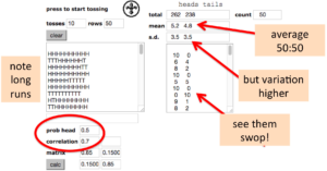
Positive correlation
If you look at the left hand text area you can see the long runs of heads and tails. Sometimes they do alternate, but then stay the same for long periods.
Looking up to the summary statistics area the average numbers of heads and tails is near 50:50 — the coin was fair, but the standard deviation is a lot higher than in the independent case. This is very evident if you look at the right-hand text area with the totals as they swing between extreme values much more than the independent coin did (even more that its quite wild randomness!).
Negative correlation
Finally we can enter a negative value for the correlation (below) to see the opposite effect.
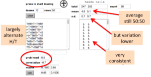
Negative correlation
Now the rows of Hs and Ts alternate a lot of time, far more than a normal coin.
The average is still close to 50:50, but this time the variation is lower and you can see this in the row totals, which are typically much closer to five heads and five tails than the ordinary coin.
Recall the gambler’s fallacy that if a coin has fallen heads lots of times it is more likely to be a tail next. In some way this coin is a bit like that, effectively evening out the odds, hence the lower variation.