 The heart of gaining power in your studies is understanding the noise–effect–number triangle. Power arises from a combination of the size of the effect you are trying to detect, the size of the study (number of trails/participants) and the size of the ‘noise’ (the random or uncontrolled factors). We can increase power by addressing any one of these.
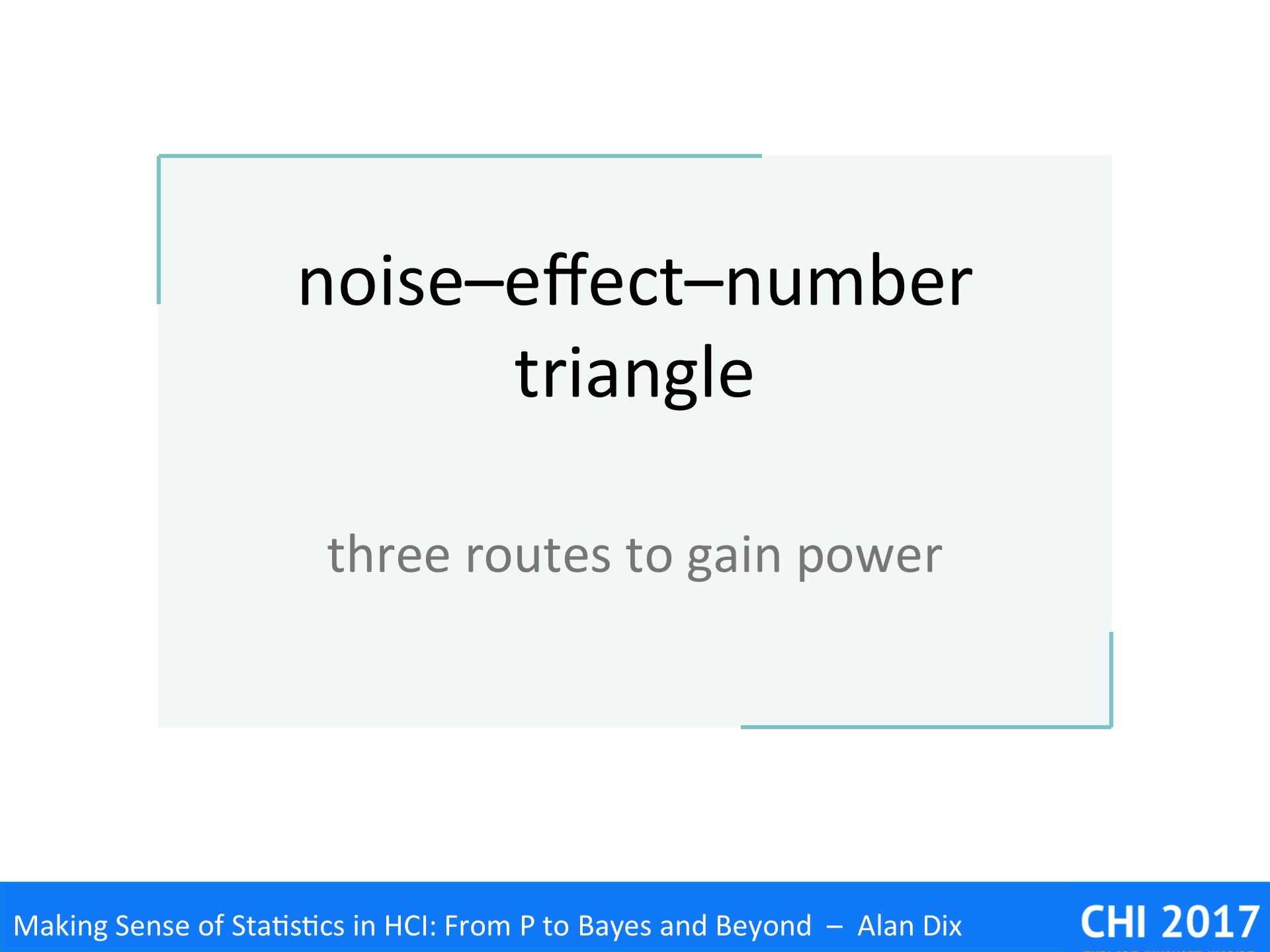
Cast your mind back to your first statistics course, or when you first opened a book on statistics.
The standard deviation (sd) is one of the most common ways to measure of the variability of a data point. This is often due to ‘noise’, or the things you can’t control or measure.
For example, the average adult male height in the UK is about 5 foot 9 inches ( with a standard deviation of about 3 inches (7.5cm), most British men are between 5′ 6″ (165cm) and 6′ (180cm) tall.
However, if you take a random sample and look at the average (arithmetic mean), this varies less as typically your sample has some people higher than average, and some people shorter than average, and they tend to cancel out. The variability of this average is called the standard error of the mean (or just s.e.), and is often drawn as little ‘error bars’ on graphs or histograms, to give you some idea of the accuracy of the average measure.
You might also remember that, for many kinds of data the standard error of the mean is given by:
s.e. = σ / √n (or if σ is an estimate √n-1 )
For example, of you have one hundred people, the variability of the average height is one tenth the variability of a single person.
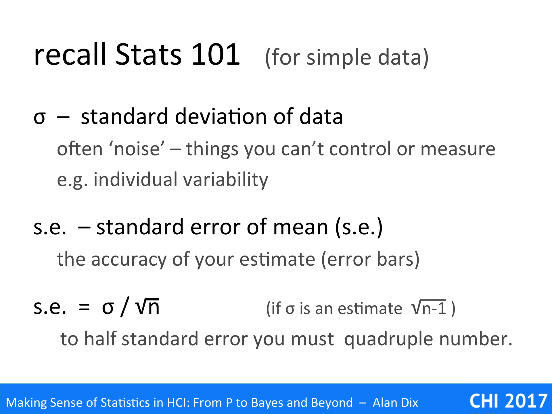
The question you then have to ask yourself is how big an effect do you want to detect? Imagine I am about to visit Denmark. I have pretty good idea that Danish men are taller than British men and would like to check this. If the average were a foot (30cm) I definitely want to know as I’ll end up with a sore neck looking up all the time, but if it is just half an inch (1.25cm) I probably don’t care.
Let’s call this least difference that I care about δ (Greek letters, it’s a mathematician thing!), so in the example δ = 0.5 inch.
If I took a sample of 100 British men and 100 Danes, the standard error of the mean would be about 0.3 inch (~1cm) for each, so it would be touch and go if I’d be able to detect the difference. However, if I took a sample of 900 of each, then the s.e. of each average would be about 0.1 inch, so I’d probably be easily able to detect differences of 0.5 inch.
In general, we’d like the minimum difference we want to detect to be substantially bigger than the standard error of the mean in order to be able to detect the difference. That is:
δ >> σ / √n
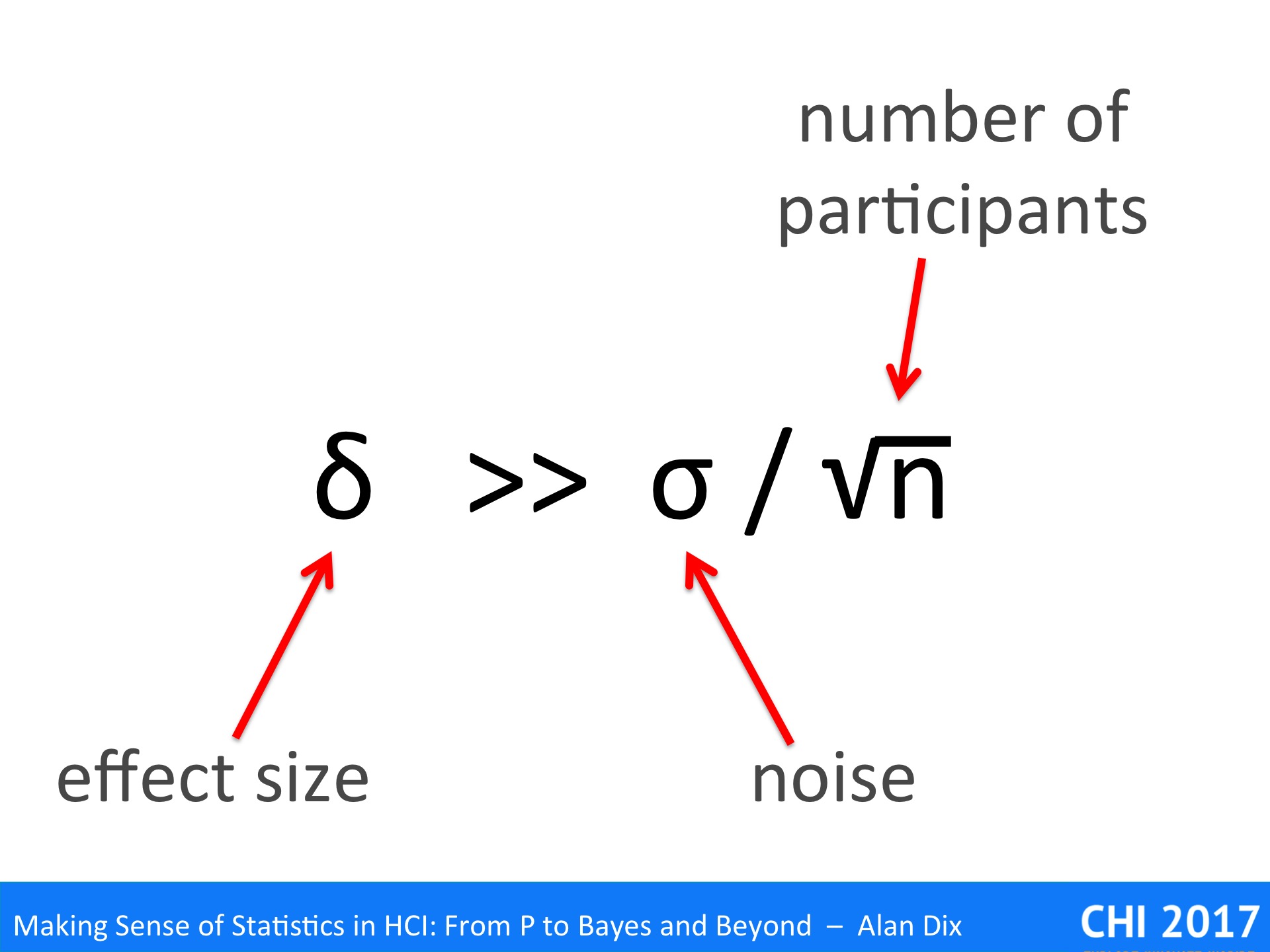
Note the three elements here:
- the effect size
- the amount of noise or uncontrolled variation
- the number of participants, groups or trials
Although the meanings of these vary between different kinds of data and different statistical methods, the basic triad is similar. This is even in data, such as network power-law, where the standard deviation is not well defined and other measures of spread or variation apply (Remember that this is a different use of the term ‘power’). In such data it is not the square root of participants that is the key factor, but still the general rule that you need a lot more participants to get greater accuracy in measures … only for power law data the ‘more’ is even greater than squaring!

Once we understand that statistical power is about the relationship between these three factors, it becomes obvious that while increasing the number of subjects is one way to address power, it is not the only way. We can attempt to effect any one of the three, or indeed several while designing our user studies or experiments.
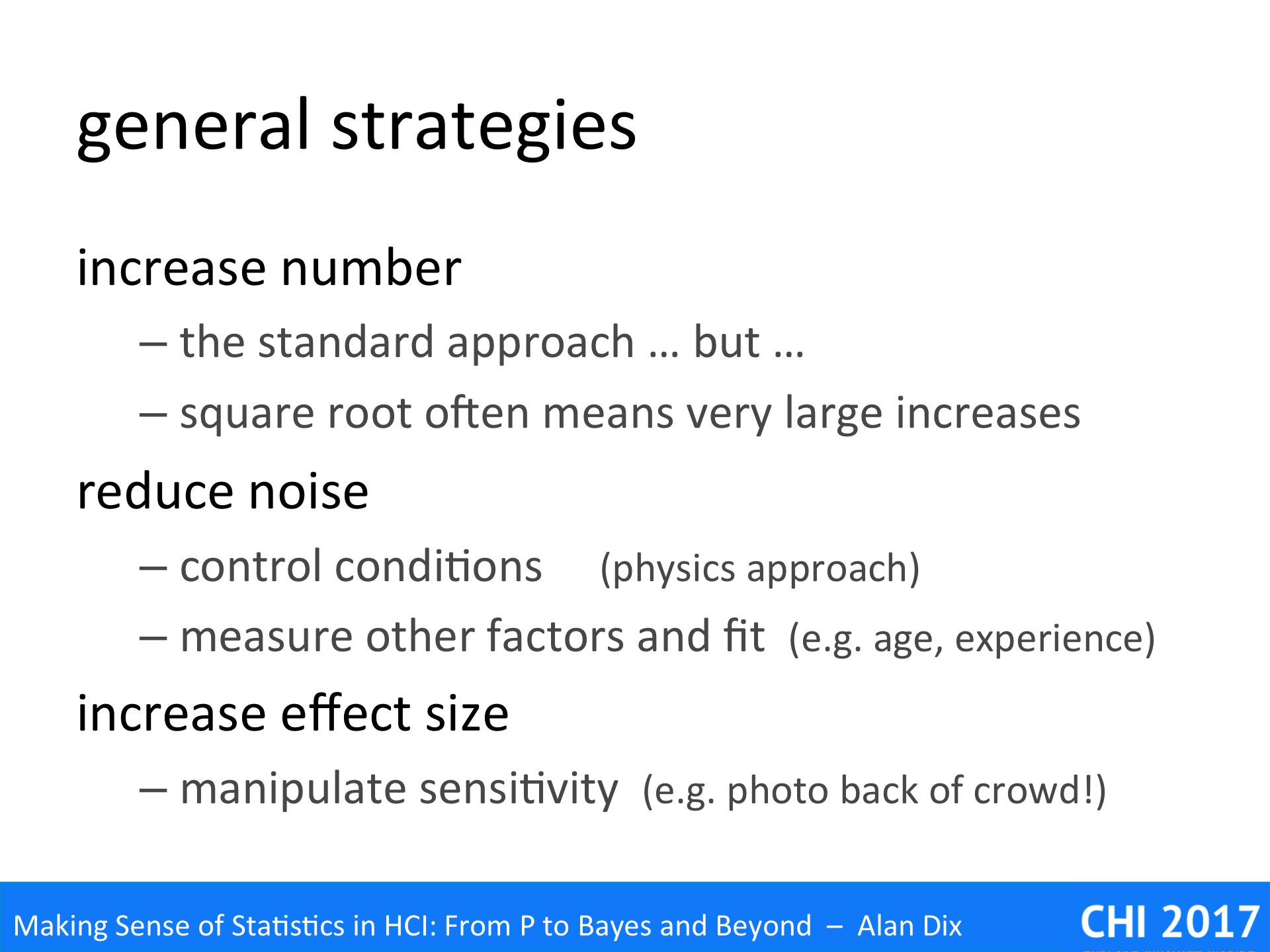
Thinking of this we have three general strategies:
- increase number – As mentioned several times, this is the standard approach, and the only one that many people think about. However, as we have seen, the square root means that we often need very lareg increase in the number of subjects or trials in order to reduce the variability of our results to acceptable level. Even when you have addressed other parts of the noise–effect–number triangle, you still have to ensure you have sufficient subjects, although hopefully less than you would need by a more naïve approach.
- reduce noise – Noise is about variation due to actors that you do not control or know about; so, we can attempt to attack either of these. First we can control conditions reducing the variability in our study; this is the approach usually take in physics and other sciences, using very pure substances, with very precise instruments in controlled environments. Alternatively, we can measure other factors and fit or model the effect of these, for example, we might ask the participants’ age, prior experience, or other things we think may affect the results of our study.
- increase effect size – Finally, we can attempt to manipulate the sensitivity of our study. A notable example of this is the photo from the back of the crowd at President Trump’s inauguration. It was very hard to assess differences in crowd size at different events from the photos taken from the front of the crowd, but photos at the back are a far more sensitive. Your studies will probably be less controversial, but you can use the same technique. Of course, there is a corresponding danger of false baselines, in that we may end up with a misleading idea of the size of effects — as noted previously with power comes the responsibility to report fairly and accurately.
In the following two posts, we will consider strategies that address the factors of the noise–effect–number triangle in different ways. We will concentrate first on the subjects, the users or participants in our studies, and then on the tasks we give them to perform.