 This part will begin with some exercises and demonstrations of the unexpected wildness of random phenomena including the effects of bias and non-independence (when one result effects others).
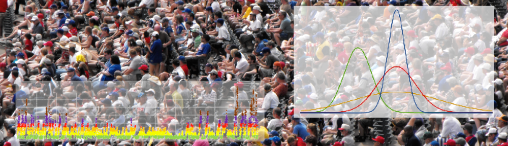
We will discuss different kinds of distribution and the reasons why the normal distribution (classic hat shape), on which so many statistical tests are based, is so common. In particular we will look at some of the ways in which the effects we see in HCI may not satisfy the assumptions behind the normal distribution.
Most will be aware of the use of non-parametric statistics for discrete data such as Likert scales, but there are other ways in which non-normal distributions arise. Positive feedback effects, which give rise to the beauty of a snowflake, also create effects such as the bi-modal distribution of student marks in certain kinds of university courses (don’t believe those who say marks should be normally distributed!). This can become more complex if feedback processes include some form of threshold or other non-linear effect (e.g. when the rate of a task just gets too much for a user).
All of these effects are found in the processes that give rise to social networks both online and offline and other forms of network phenomena, which are often far better described by a long-tailed ‘power law’.
Just how random is the world?
We often underestimate just how wild random phenomena are – we expect to see patterns and reasons for what is sometimes entirely arbitrary.
Through a story and some exercises, I hope that you will get a better feel for how wild randomness is. We sometimes expect random things to end up close to their average behaviour, but we’ll see that variability is often large.
When you have real data you have a combination of some real effect and random ‘noise’. However, by doing some coin tossing experiments you know that the coins you are dealing with are near enough fair – everything you see will be sheer randomness.
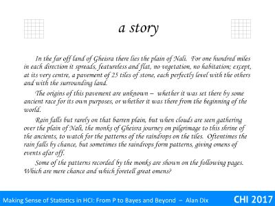
We’ll start with a story:
In the far off land of Gheisra there lies the plain of Nali. For one hundred miles in each direction it spreads, featureless and flat, no vegetation, no habitation; except, at its very centre, a pavement of 25 tiles of stone, each perfectly level with the others and with the surrounding land.
The origins of this pavement are unknown – whether it was set there by some ancient race for its own purposes, or whether it was there from the beginning of the world.
Rain falls but rarely on that barren plain, but when clouds are seen gathering over the plain of Nali, the monks of Gheisra journey on pilgrimage to this shrine of the ancients, to watch for the patterns of the raindrops on the tiles. Oftentimes the rain falls by chance, but sometimes the raindrops form patterns, giving omens of events afar off.
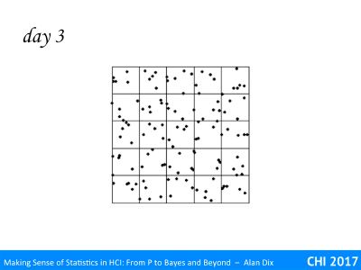
Some of the patterns recorded by the monks are shown on the following slides. Which are mere chance and which foretell great omens?
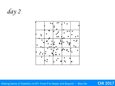

Before reading on make your choices and record why you made your decision.

Just a reminder choose first and then read one 😉
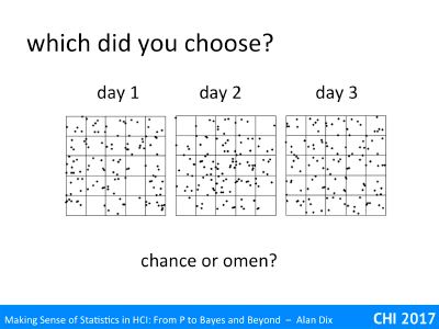
Before, revealing the true omens, you might like to know how you fare alongside three and seven year olds.
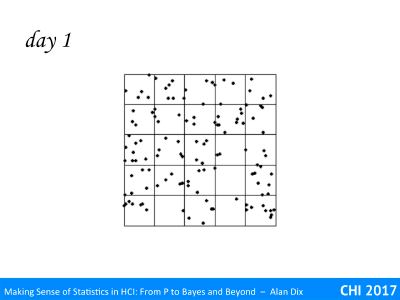
When very young children are presented with this choice they give very mixed answers, but have a small tendency to think that distributions like day 1 are real rainfall, whereas those like day 3 are an omen.
In contrast, once children are older, seven or so, they are more consistent and tended to plump for day 3 as the random rainfall.
Were you more like the three year old and thought day 1 was random rainfall, or more like the seven year old and thought day 1 was an omen and day 3 random. Or perhaps you were like neither of them and thought day 2 was true random rainfall.
Let’s see who is right.
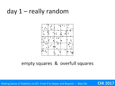
When you looked at day 1 you might have seen a slight diagonal tendency with the lower right corner less dense then the upper left. Or you may have noted the suspiciously collinear three dots in the second tile on the top row.
However, this pattern, the preferred choice f the three year od, is in fact the random rainfall – or at least as random as a computer random number generator can manage!
In true random phenomena you often do get gaps, dense spots or apparent patterns, but this is just pure chance.
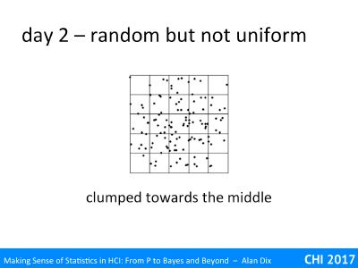
In day 2 you might have thought it looked a little clumped towards the middle.
In fact this is perfectly right, it is exactly the same tiles as in day 1, but re-ordered so that the fuller tiles are towards the centre, and the part-empty ones to the edges.
This is an omen!

Finally, day 3 is also an omen.
This is the preferred choice of seven year olds as being random rainfalls and also, I have found, the preferred choice of 27, 37 and 47 year olds.
However it is too uniform. The drops on each tile are distributed randomly, but there are precisely five drops on each tile.
At some point during our early education we ‘learn’ (wrongly!) that random phenomena are uniform. Although this is nearly true when there are very large numbers involved (maybe 12,500 drops rather than 125), wth smaller numbers the effects are far more wacky than one might imagine.
Now for a different exercise, and this time you don’t just have to choose, you have to do something.
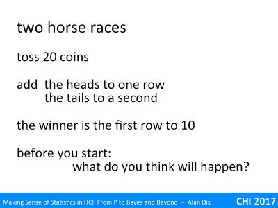
Find a coin, or even better if you have 20, get them.
Toss the coins one by one and put the heads into one row and the tails into another.
Keep on tossing until one line of coins has ten coins in it … you could even mark a finish line 10 coins away from the start.
If you only have one coin you’ll have to just toss it and keep tally!
If you are on your own repeat this several times.
However, before you start think about what you expect to see.
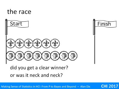
So what happened?
Did you get a clear winner, or were they neck and neck?
And what did you expect to happen?
I had a go and did five races. In one case they were nearly neck-and-neck at 9 heads to 10 tails, but the other four races were won by heads with some quite large margins: 10 to 7, 10 to 6, 10 to 5 and 10 to 4.
Often people are surprised because they are expecting a near neck and neck race every time. As the coins are all fair, they expect approximately equal numbers of heads and tails. However, just like the rainfall in Gheisra, it is very common to have one quite far ahead of the other.
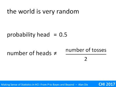
In your head you might think that because the probability of it being a head is a half, the number of heads will be near enough half. Indeed, this is the case if you average over lots and lots of tosses. However, with just 20 coins in a race, the variability is large.
The probability of getting an outright winner all heads or all tails is low, only about one in five hundred. However, the probability of getting a near wipe-out with one head and ten tails or vice versa is around one in fifty – in a large class one person is likely to have this.
I hope these two activities begin to give some idea of the wild nature of random phenomena. We can see a few general lessons.
First apparent patterns or differences may just be pure chance. For example, if you had found heads winning by 10 to 2, you might have thought this meant that your coin was in some way biased t heads, or you might have thought that the nearly straight line of three drops on day 1 had to mean something. But random things are so wild that sometimes apparently systematic effects happen by chance.
It is also remembering that this wildness may lead to what appear to be ‘bad values’. If you had got 10 tails and just 1 head, you might have thought “but coins are fair, so I must have done something wrong”.
Famous scientists have fallen for this fallacy!
Mendel’s experiment on inheritance of sweet pea characteristics laid the foundations for modern genetics. However, his results are a little too good. If you cross-pollinate two plants one pure bred to have a recessive characteristic and one purely dominant, you expect to see the second generation to have observable characteristics that are dominant and recessive in the ration 3:1. In Mendel’s data the ratios are just a little too close to this figure. It seems likely that he rejected ‘bad values’ assuming he had done something wrong when in fact they were just the results of chance.
The same thing can happen in Physics. In 1909 Millikan and Harvey Fletcher did an experiment that showed that each electron has an identical charge and measure it (also known as the ‘Millikan can experiment’). To do this they created charged oil drops and suspended them using their electrical charge. The relationship between the field needed and size (and hence weight) of the drop enabled them to calculate the charge on each oil drop. These always came in multiples of a single value – the electron charge. Only there are sources of error in all the measurements and yet the reported charges are a little too close to multiples of the same number. Again it looks like ‘bad’ results were ignored as some form of mistake during the setup of the experiment.