When you take a measurement, whether it is the time for someone to complete a task using some software, or a preferred way of doing something, you are using that measurement to find out something about the ‘real’ world – the average time for completion, or the overall level of preference amongst you users.

Two of the core things you need to know is about bias (is it a fair estimate of the real value) and variability (how likely is it to be close to the real value).

The word ‘bias’ in statistics has a precise meaning, but it is very close to its day-to-day meaning.

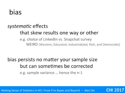
Bias is about systematic effects that skew your results in one way or another. In particular, if you use your measurements to predict some real world effect, is that effect likely to over or under estimate the true value; in other words, is it a fair estimate.

Say you take 20 users, and measure their average time to complete some task. You then use that as an estimate of the ‘true’ value, the average time to completion of all your users. Your particular estimate may be low or high (as we saw with the coin tossing experiments). However, if you repeated that experiment very many times would the average of your estimates end up being the true average?

If the complete user base were employees of a large company, and the company forced them to work with you, you could randomly select your 20 users, and in that case, yes, the estimate based on the users would be unbiased¹.

However, imagine you are interested in popularity of Justin Bieber and issued a survey on a social network as a way to determine this. The effects would be very different if you chose to use LinkedIn or WhatsApp. No matter how randomly you selected users from LinkedIn, they are probably not representative of the population as a whole and so you would end up with a biased estimate of his popularity.

Crucially, the typical way to improve an estimate in statistics is to take a bigger sample: more users, more tasks, more tests on each user. Typically, bias persists no matter the sample size².

However, the good news is that sometimes it is possible to model bias and correct for it. For example, you might ask questions about age or other demographics’ and then use known population demographics to add weight to groups under-represented in your sample … although I doubt this would work for the Justin Beiber example: if there are 15 year-old members of linked in, they are unlikely to be typical 15-year olds!

If you have done an introductory statistics course you might have wondered about the ‘n-1’ that occurs in calculations of standard deviation or variance. In fact this is precisely a correction of bias, the raw standard deviation of a sample slightly underestimates the real standard deviation of the overall population. This is pretty obvious in the case n=1 – imagine grabbing someone from the street and measuring their height. Using that height as an average height for everyone, would be pretty unreliable, but it is unbiased. However, the standard deviation of that sample of 1 is zero, it is one number, there is no spread. This underestimation is less clear for 2 or more, but in larger samples it persists. Happily, in this case you can precisely model the underestimation and the use of n-1 rather than n in the formulae for estimated standard deviation and variance precisely corrects for the underestimation.

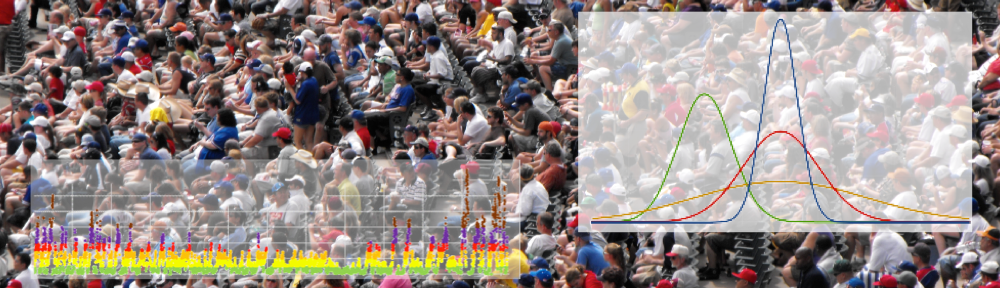
If you toss 10 coins, there is only a one in five hundred chance of getting either all heads or all tails, about a one in fifty chance of getting only one head or one tails, the really extreme values are relatively unlikely. However, there about a one in ten chance of getting either just two heads or two tails. However, if you kept tossing the coins again and again, the times you got 2 heads and 8 tails would approximately balance the opposite and overall you would find that the average proportion of heads and tails would come out 50:50.

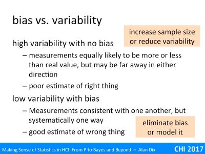
That is the proportion you estimate by tossing just 10 coins has a high variability, but is unbiased. It is a poor estimate of the right thing.

Often the answer is to just take a larger sample – toss 100 coins or 1000 coins, not just 10. Indeed when looking for infrequent events, physicists may leave equipment running for months on end taking thousands of samples per second.

You can sample yourself out of high variability!

Think now about studies with real users – if tossing ten coins can lead to such high variability; what about those measurements on ten users?

In fact for there may be time, cost and practicality limits on how many users you can involve, so there are times when you can’t just have more users. My ‘gaining power’ series of videos includes strategies including reducing variability for being able to obtain more traction form the users and time you have available.

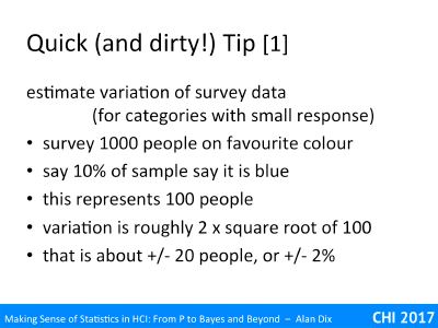
In contrast, let’s imagine you have performed a random survey of 10,000 LinkedIn users and obtained data on their attitudes to Justin Beiber. Let’s say you found 5% liked Justin Beiber’s music. Remembering the quick and dirty rule³, the variability on this figure is about +/- 0.5%. If you repeated the survey, you would be likely to get a similar answer.

That’s is you have a very reliable estimate of his popularity amongst all LinkedIn users, but if you are interested in overall popularity, then is this any use?

You have a good estimate of the wrong thing.

As we’ve discussed you cannot simply sample your way out of this situation, if your process is biased it is likely to stay so. In this case you have two main options. You may try to eliminate the bias – maybe sample over a wide range of social network that between them offer a more representative view of society as whole.   Alternatively, you might try to model the bias, and correct for it.

On the whole high variability is a problem, but has relatively straightforward strategies for dealing with. Bias is your real enemy!

1. Assuming they behaved as normal in the test and weren’t annoyed at being told to be ‘volunteers’. [↩]
2. Actually there are some forms of bias that do go away with large samples, called asymptotically unbiased estimators, but this does not apply in the cases where the way you choose your sample has created an unrepresentative sample, or the way you have set up your study favours one outcome. [↩]
3. 5% of 10,000 represents 500 users.  The square root of 500 is around 22, twice that a bit under 50, so our estimate of variability is 500+/–50, or, as a percentage of users,  5% +/– 0.5% [↩]

We often deal with survey or count data. This might come in public forms such as opinion poll data preceding an election, or from your own data when you email out a survey, or count kinds of errors in a user study.

So when you find that 27% of the users in your study had a problem, how confident do you feel in using this to estimate the level of prevalence amongst users in general? If you did a bigger study wit more users would you be surprised if the figure you got was actually 17%, 37% or 77%?

You can work out precise numbers of this, but in this video I’ll give a simple rule of thumb method for doing a quick estimate.

We’re going to deal with this by looking at three separate cases.

First when the number you are dealing with is a comparatively small proportion of the overall sample.

For example, assume you want to know about people’s favourite colours. You do a survey of 1000 people at 10% say their favourite colour is blue. The question is how reliable this figure is. If you had done a larger survey, would the answer be close to 10% or could it be very different?

The simple rule is that the variation is 2 x the square root number of people who chose blue.

To work this out first calculate how many people the 10% represents. Given the sample was 1000, this is 100 people. The square root of 100 is 10, so 2 times this is 20 people. You can be reasonably confident (about 95%) that the number of people choosing blue in your sample is within +/- 20 of the proportion you’d expect from the population as a whole. Dividing that +/-20 people by the 1000 sample, the % of people for whom blue is their favourite colour is likely to be within +/- 2% of the measured 10%.

The second case is when you have a large majority who have selected a particular option.

For example, let’s say in another survey, this time of 200 people, 85% said green was their favourite colour.

This time you still apply the “2 x square root” rule, but instead focus on the smaller number, those who didn’t choose green. The 15% who didn’t choose green is 15% of 200 that is 30 people. The square root of 30 is about 5.5, so the expected variability is about +-11, or in percentage terms about +/- 5.5%.

That is the real proportion over the population as a whole could be anywhere between 80% and 90%.

Notice how the variability of the proportion estimate from the sample increases as the sample size gets smaller.

Finally if the numbers are near the middle, just take the square root, but this time multiply by 1.5.

For example, if you took a survey of 2000 people and 50% answered yes to a question, this represents 1000 people. The square toot of 1000 is a bit over 30, so 1.5 times this is around 50 people, so you expect a variation of about +/- 50 people, or about +/- 2.5%.

Opinion polls for elections often have samples of around 2000, so if the parties are within a few points of each other you really have no idea who will win.

For those who’d like to understand the detailed stats for this (skip if you don’t!) …

These three cases are simplified forms of the precise mathematical formula for the variance of a Binomial distribution np(1-p), where n is the number in the sample and p the true population proportion for the thing you are measuring. When you are dealing with fairly small proportions the 1-p term is close to 1, so the whole variance is close to np, that is the number with the given value. You then take the square root to give the standard deviation. The factor of 2 is because about 95% of measurements fall within 2 standard deviations. The reason this becomes 1.5 in the middle is that you can no longer treat (1-p) as nearly 1, and for p =0.5, this makes things smaller by square root of 0,5, which is about 0.7. Two times 0,7 is (about) one and half (I did say quick and dirty!).

However, for survey data, or indeed any kind of data, these calculations of variability are in the end far less critical than ensuring that the sample really does adequately measure the thing you are after.

Is it fair? – Has the way you have selected people made one outcome more likely. For example, if you do an election opinion poll of your Facebook friends, this may not be indicative of the country at large!

For surveys, has there been self-selection? – Maybe you asked a representative sample, but who actually answered. Often you get more responses from those who have strong feelings about the issue. For usability of software, this probably means those who have had a problem with it!

Have you phrased the question fairly? – For example, people are far more likely to answer “Yes” to a question, so if you ask “do you want to leave?” you might get 60% saying “yes” and 40% saying no, but if you asked the question in the opposite way “do you want to stay?”, you might still get 60% saying “yes”.