 You use statistics when there is something in the world you don’t’ know, and want to get a level of quantified understanding of it based on some form of the measurement or sample.
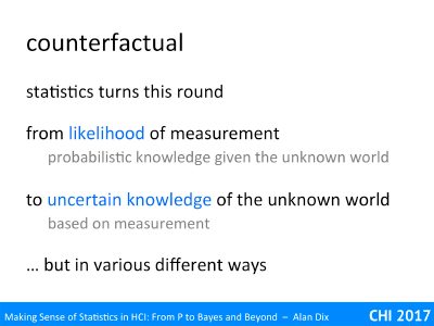
One key mathematical element of this shared by all techniques is the idea of conditional probability and likelihood; that is the probability of a specific measurement occurring assuming you know everything pertinent about the real world. Of course the whole point is that you don’t know what is true of the real world, but do know about the measurement, so you need to do back-to-front counterfactual reasoning, to go back from measurement to the world!
Future videos will discuss three major kinds of statistical analysis methods:
- Hypothesis testing (the dreaded p!) – robust but confusing
- Confidence intervals – powerful but underused
- Bayesian stats – mathematically clean but fragile
The first two use essentially the same theoretical approach, and the difference is more about the way you present results. Bayesian statistics takes a fundamentally different approach, with its own strengths and weaknesses.

First of all let’s recall the ‘job of statistics‘, which is an attempt to understand the fundamental properties of the real world based on measurements and samples. For example, you may have taken a dozen people (the sample), asked them to perform a task on a piece of software and a new version of the software. You have measured response times, satisfaction, error rate, etc., (the measurement) and want to know whether your new software will out perform the original software for the whole user group (the real world).
We are dealing with data with a lot of randomness and so need to deal with probabilities, but in particular what is known as conditional probability.
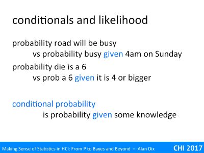
Imagine the main street of a local city. What is the probability that it is busy?
Now imagine that you are standing in the same street but it is 4am on a Sunday morning: what is the probability it is busy given this?
Although the overall probability of it being busy (at a random time of day) is high, the probability that it is busy given it is 4am on a Sunday is lower.
Similarly think of a throwing single die. What is the probability it is a six? 1 in 6.
However, if I peek and tell you it is at least 4. What now is the probability it is a six? The probability it is a six given it is four or greater is 1 in 3.
When we have more information, then we change our assessment of the probability of events accordingly. This calculation of probability given some information is what mathematicians call conditional probability.
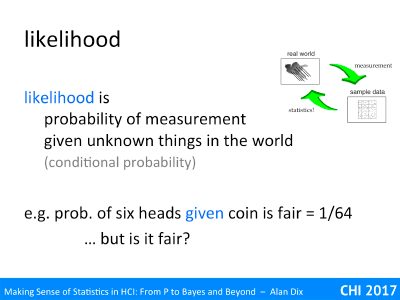
Returning to the job of statistics, we are interested in the relationship between measurements of the real world and what is true of the real world. Although we may not know what is true of the world (what is the actual error rate of our new software going to be), we can often work out the probability of measurements given (the unknown) state of the world.
For example, if the probability of a user making a particular error is 1 in 10, then the probability that exactly 3 make the error out of a sample of 5 is 7.29% (calculated from the Binomial distribution).
This conditional probability of a measurement given the state of the world (or typically some specific parameters of the world) is what statisticians call likelihood.
As another example the probability that six tosses of a coin will come out heads given the coin is fair is 1/64, or in other words the likelihood that it is fair is 1/64. If instead the coin were biased 2/3 heads 1/3 tails, the probability of 6 heads given this, likelihood fo the coin having this bias, is 64/729 ~ 1/ 11.
Note this likelihood is NOT the probability that the coin is fair or biased, we may have good reason to believe that most coins are fair. However, it does constitute evidence. The core difference between different kinds of statistics is the way this evidence is used.
Effectively statistics tries to turn this round, to take the likelihood, the probability of the measurement given the unknown state of the world, and reverse this, use the fact that the measurement has occurred to tell us something about the world.
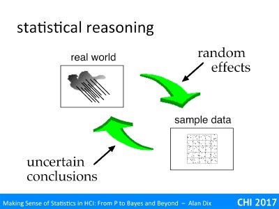
Going back again to the job of statistics, the measurements we have of the world are prone to all sorts of random effects. The likelihood models the impact of these random effects as probabilities. The different types of statistics then use this to produce conclusions about the real world.
However, crucially these are always uncertain conclusions. Although we can improve our ability to see through the fog of randomness, there is always the possibility that by shear chance things appear to suggest one conclusion even though it is not true.

We will look at three types of statistics.
Hypothesis testing is what you are most likely to have seen – the dreaded p! It was originally introduced as a form of ‘quick hack’, but has come to be the most widely used tool. Although it can be misused, deliberately or accidentally, in many ways, it is time-tested, robust and quite conservative. The downside is that understanding what it really says (not p<5% means true!) can be slightly complex.
Confidence intervals use the same underlying mathematical methods as hypothesis testing, but instead of taking about whether there is evidence for or against a single value, or proposition, confidence intervals give a range of values. This is really powerful in giving a sense of the level of uncertainty around an estimate or prediction, but are woefully underused.
Bayesian statistics use the same underlying likelihood (although not called that!) but combine this with numerical estimates of the probability of the world. It is mathematically very clean, but can be fragile. One needs to be particularly careful to avoid conformation bias and when dealing with multiple sources of non-independent evidence. In addition, because the results are expressed as probabilities, this may give an impression of objectivity, but in most cases it is really about modifying one’s assessment of belief.
We will look at each of these in more detail in coming videos.
To some extent these techniques have been pretty much the same for the past 50 years, however computation has gradually made differences. Crucially, early statistics needed to relatively easy to compute by hand, whereas computer-based statistical analyses can use more complex methods. This has allowed more complex models based on theoretical distributions, and also simulation methods that use models where there is no ‘nice’ mathematical solution.