Significance testing helps us to tell the difference between a real effect and random-chance patterns, but it is less helpful in giving us a clear idea of the potential size of an effect, and most importantly putting bounds on how similar things are. Confidence intervals help with both of these, giving some idea of were real values or real differences lie.

 

So you ran your experiment, you compared user response times to a suite of standard tasks, worked out the statistics and it came out not significant – unproven.

As we’ve seen this does not allow us to conclude there is no difference, it just may be that the difference was too small to see given the level of experimental error. Of course this error may be large, for example if we have few participants and there is a lot of individual difference; so even a large difference may be missed.

How can we tell the difference between not proven and no difference?

In fact it is usually impossible to say definitively ‘no difference’ as it there may always be vanishingly small differences that we cannot detect. However, we can put bounds on inequality.

A confidence interval does precisely this. It uses the same information and mathematics as is used to generate the p values in a significance test, but then uses this to create a lower and upper bound on the true value.

For example, we may have measured the response times in the old and new system, found an average difference of 0.3 seconds, but this did not turn out to be a statistically significant difference.

On its own this simply puts us in the ‘not proven’ territory, simply unknown.

However we can also ask our statistics application to calculate a 95% confidence interval, let’s say this turns out to be [-0.7,1.3] (often, but not always, these are symmetric around the average value).

Informally this gives an idea of the level of uncertainty about the average. Note this suggests it may be as low as -0.7, that is our new system maybe up to 0.7 second slower that the old system, but also may be up to 1.3 seconds faster.

However, like everything in statistics, this is uncertain knowledge.

What the 95% confidence interval actually says that is the true value were outside the range, then the probability of seeing the observed outcome is less than 5%. In other words if our null hypothesis had been “the difference is 2 seconds” or “the difference is 1.4 seconds”, or “the difference is 0.8 seconds the other way”, all of these cases the probability of the outcome would be less than 5%.

By a similar reasoning to the significance testing, this is then taken as evidence that the true value really is in the range.

Of course, 5% is a low degree of evidence, maybe you would prefer a 99% confidence interval, this then means that of the true value were outside the interval, the probability of seeing the observed outcome is less than 1 in 100. This 99% confidence interval will be wider than the 95% one, perhaps [-1,1.6], if you want to be more certain that the value is in a range, the range becomes wider.

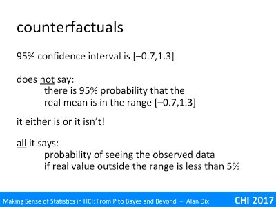
Just like with significance testing, the 95% confidence interval of [-0.7,1.3] does not say that there is a 95% probability that the real value is in the range, it either is or it is not.

All it says is that if the real value were to lie outside the range, then the probability of the outcome is less than 5% (or 1% for 99% confidence interval).

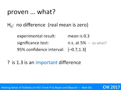
Let’s say we have run our experiment as described and it had a mean difference in response time of 0.3 seconds, which was not significant, even at 5%. At this point, we still had no idea of whether this meant no (important) difference or simply a poor experiment. Things are inconclusive.

However, we then worked out the 95% confidence interval to be [-0.7,1.3]. Now we can start to make some stronger statements.

The upper limit of the confidence interval is 1.3 seconds; that is we have a reasonable level of confidence that the real difference is no bigger than this – does it matter, is this an important difference. Imagine this is a 1.3 second difference on a 2 hour task, and that deploying the new system would cost millions, it probably would not be worth it.

Equally, if there were other reasons we want to deploy the system would it matter if it were 0.7 seconds slower?

We had precisely this question with a novel soft keyboard for mobile phones some years ago [HD04]. The keyboard could be overlaid on top of content, but leaving the content visible, so had clear advantages in that respect over a standard soft keyboard that takes up the lower part of the screen.   My colleague ran an experiment and found that the new keyboard was slower (by around 10s in a 100s task), and that this difference was statistically significant.

If we had been trying to improve the speed of entry this would have been a real problem for the design, but we had in fact expected it to be a little slower, partly because it was novel and so unfamiliar, and partly because there were other advantages. It was important that the novel keyboard was not massively slower, but a small loss of speed was acceptable.

We calculated the 95% confidence interval for the slowdown at [2,18]. That is we could be fairly confident it was at least 2 seconds slower, but also confident that it was no more than 18 seconds slower.

Note this is different from the previous examples, here we have a significant difference, but using the confidence interval to give us an idea of how big that difference is. In this case, we have good evidence that the slow down was no more than about 20%, which was acceptable.

Researchers are often more familiar with significance testing and know that the need to quote the number of participants, the test used, etc.; you can see this in every other report you gave read that uses statistics.

When you quote a confidence level the same applies. If the data is two-outcome true/false data (like the coin toss), then the confidence interval may have been calculated using the Binomial distribution, if it is people’s heights it might use the Normal or Students-t distribution – this needs to be reported so that others can verify the calculations, or maybe reproduce your results.

Finally do remember that, as with all statistics, the confidence interval is still uncertain. It offers good evidence that the real value is within the interval, but it could still be outside.

What you can say

In the video and slides I spend so much time warning you what is not true, I forgot to mention one of the things that you can say with certainty from a confidence interval.

If you run experiments or studies, calculate the 95% confidence interval for each and then work on the assumption that the real value lies in the range, then at least 95% of the time you will be right.

Similarly if you calculate 99% confidence intervals (usually much wider) and work on the assumption that the real value lies in the rage, then at least 99% of the time you will be right.

This is not to say that for any given experiment the probability of the real value lies in the range, it either does or doesn’t. just puts a limit on the probability you are wrong if you make that assumption.  These sound almost the same, but the former is about the real value of something that may have no probability associated with it; it is just unknown; the latter is about the fact that you do lots of experiments, each effectively each like the toss of a coin.

So if you assume something is in the 95% confident range, you really can be 95% confident that you are right.

Of course, this is about ALL of the experiments that you or others do .  However, often only positive results are published; so it is NOT necessarily true of the whole published literature.

References

[HD04] J. Hudson, A. Dix and A. Parkes (2004). User Interface Overloading, a Novel Approach for Handheld Device Text Input. Proceedings of HCI2004, Springer-Verlag. pp. 69-85. http://www.alandix.com/academic/papers/HCI2004-overloading/