 Bayesian reasoning allows one to make strong statements about the probability of things based on evidence. This can be used for internal algorithms, for example, to make adaptive or intelligent interfaces, and also for a form of statistical reasoning that can be used as an alternative to traditional hypothesis testing.
However, to do this you need to be able to quantify in a robust and defensible manner what are the expected prior probabilities of different hypothesis before an experiment. This has potential dangers of confirmation bias, simply finding the results you thought of before you start, but when there are solid grounds for those estimates it is precise and powerful.
Crucially it is important to remember that Bayesian statistics is ultimately about quantified belief, not probability.
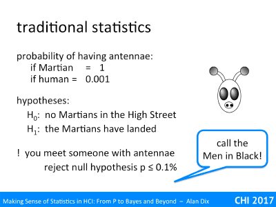
It is common knowledge that all Martians have antennae (just watch a sci-fi B-movie). However, humans rarely do. Maybe there is some rare genetic condition or occasional fancy dress, so let’s say the probability that a human has antennae is no more than 1 in a 1000.
You decide to conduct a small experiment. There are two hypotheses:
H0 – there are no Martians in the High Street
H1 – the Martians have landed
You go out into the High Street and the first person you meet has antennae. The probability of this occurring given the null hypothesis that there are no Martians in the High Street is 1 in 1000, so we can reject the null hypothesis at p<=0.1% … which is a far stronger result than you likely to see in most usability experiments.
Should you call the Men in Black?
For a more familiar example, let’s go back to the coin tossing. You pull a coin out of your pocket, toss it 10 times and it is a head every time. The chances of this given it is a fair coin is just 1 in 1000; do you assume that the coin is fixed or that it is just a fluke?
Instead imagine it is not a coin from your pocket, but a coin from a stall-holder at a street market doing a gambling game – the coin lands heads 10 times in a row, do you trust it?
Now imagine it is a usability test and ten users were asked to compare your new system that you have spent many weeks perfecting with the previous system. All ten users said they prefer the new system … what do you think about that?

Clearly in day-to-day reasoning we take into account our prior beliefs and use that alongside the evidence from the observations we have made.
Bayesian reasoning tries to quantify this. You turn that vague feeling that it is unlikely you will meet a Martian, or unlikely the coin is biased, into solid numbers – a probability.
Let’s go back to the Martian example. We know we are unlikely to meet a Martiona, but how unlikely. We need to make an estimate of this prior probability, let’s say it is a million to one.
prior probability of meeting a Martian = 0.000001
prior probability of meeting a human = 0.999999
Remember that the all Martians have antennae so the probability that someone we meet has antennae given they are Martian is 1, and we said the probability of antennae given they are human was 0.001 (allowing for dressing up).
Now, just as in the previous scenario, you go out into the High Street and the first person you meet has antennae. You combine this information, including the conditional probabilities given the person is Martian or human, to end up with a revised posterior probability of each:
posterior probability of meeting a Martian ~ 0.001
posterior probability of meeting a human ~ 0.999
We’ll see and example with the exact maths for this later, but it makes sense that if it were a million times more likely to meet a human than a Martian, but a thousand times less likely to find a human with antennae, then about having a final result of about a thousand to one sounds right.
The answer you get does depend on the prior. You might have started out with even less belief in the possibility of Martians landing, perhaps 1 in a billion, in which case even after seeing the antennae, you would still think it a million times more likely the person is human, but that is different from the initial thousand to one posterior. We’ll see further examples of this later.

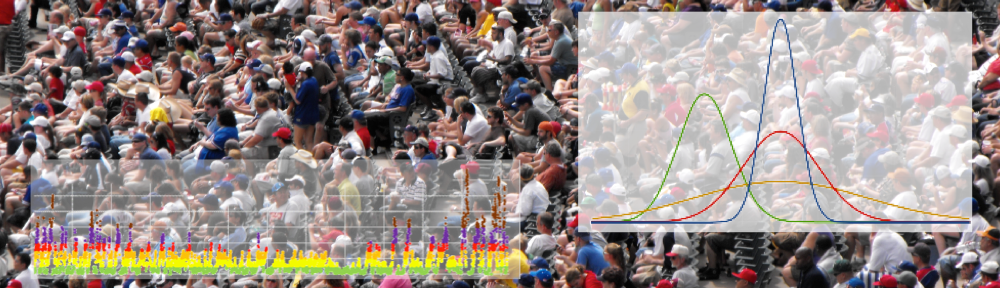
So, returning once again to the job of statistics diagram, Bayesian inference is doing the same thing as other forms of statistics, taking the sample, or measurement of the real world, which includes many random effects, and then turning this back to learn things about the real world.
The difference in Bayesian inference is that it also asks for a precise prior probability, what you would have thought was likely to be true of the real world before you saw the evidence of the sample measurements. This prior is combined with the same conditional probability (likelihood) used in traditional statistics, but because of the extra ‘information’ the result is a precise posterior distribution that says precisely how likely are different values or parameters of the real world.
The process is very mathematically sound and gives a far more precise answer than traditional statistics, but does depend on you being able to provide that initial precise prior.
This is very important, if you do not have strong grounds for the prior, as is often the case in Bayesian statistics, you are dealing with quantified belief set in the language of probability, not probabilities themselves..
We are particularly interested in the use of Bayesian methods as an alternative way to do statistics for experiments, surveys and studies. However, Bayesian inference can also be very successfully used within an application to make adaptive or intelligent user interfaces.
We’ll look at an example of how this can be used to create an adaptive website. This is partly because in this example there is a clear prior probability distribution and the meaning of the posterior is also clear. This will hopefully solidify the concepts of Bayesian techniques before looking at the slightly more complex case of Bayesian statistical inference.
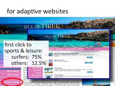
This is the front page of the Isle of Tiree website. There is a menu along the left-hand side; it starts with ‘home’, ‘about Tiree’, ‘accommodation’, and the 12th item is ‘sport & leisure’.
Imagine we have gathered extensive data on use by different groups, perhaps by an experiment or perhaps based on real usage data. We find that for most users the likelihood of clicking ‘sport & leisure’ as the first selection on the site is 12.5%, but for surfers this figure is 75%. Cleary different users access the site in different ways, so perhaps we would like to customise the site in some way for different types of users.
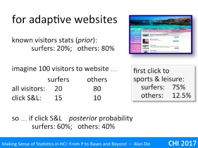
Let’s imagine we also have figures for the overall proportion of visitors to the site who are surfers or non-surfers, let’s say that the figures are 20% surfers, 80% non-surfers. Clearly, as only one in five visitors is a surfer we do not want to make the site too ‘surf-centric’.
However, let’s look at what we know after the user’s first selection.
Consider 100 visitors to the site. On average 20 of these will be surfers and 80 non-surfers. Of the 20 surfers 75%, that is 15 visitors, are likely to click ‘sorts & leisure’ first. Of the 80 non-surfers, 12.5%, that is 10 visitors are likely to click ‘sports & leisure’ first.
So in total of the 100 visitors 25 will click ‘sports & leisure’ first, Of these 15 are surfers and 10 non surfers, that is if the visitor has clicked ‘sports & leisure’ first there is a 60% chance the visitor is a surfer, so it becomes more sensible to adapt the site in various ways for these visitors. For visitors who made different first choices (and hence lower chance of being a surfer), we might present the site differently.
This is precisely the kind of reasoning that is often used by advertisers to target marketing and by shopping sites to help make suggestions.
Note here that the prior distribution is given by solid data as is the likelihood: the premises of Bayesian inference are fully met and thus the results of applying it are mathematically and practically sound.
If you’d like to see how the above reasoning is written mathematically, it goes as follows – using the notation P(A|B) as the conditional probability that A is true given B is true.
likelihood:
P( ‘sports & leisure’ first click | surfer ) = 0.75
P( ‘sports & leisure’ first click | non-surfer ) = 0.125
prior:
P( surfer ) = 0.2
P( non-surfer ) = 0.8
posterior (writing ‘S&L’ for “‘sports & leisure’ first click “) :
P( surfer | ‘S&L’ ) = P( surfer and ‘S&L’ ) / P(‘S&L’ )
where:
P(‘S&L’ ) = P( surfer and ‘S&L’ ) + P( non-surfer and ‘S&L’ )
P( surfer and ‘S&L’ ) = P(‘S&L’ | surfer ) * P( surfer )
= 0.75 * 0.2 = 0.15
P( non-surfer and ‘S&L’ ) = P(‘S&L’ | non-surfer ) * P( non-surfer )
= 0.125 * 0.8 = 0.1
so
P( surfer | ‘S&L’ ) = 0.15 / ( 0.15 + 0.1 ) = 0.6

Let’s see how the same principle is applied to statistical inference for a user study result.
Let’s assume you are comparing and old system A with your new design system B. You are clearly hoping that your newly designed system is better!
Bayesian inference demands that you make precise your prior belief about the probability of the to outcomes. Let say that you have been quite conservative and decided that:
prior probability A & B are the same: 80%
prior probability B is better: 20%
You now do a small study with four users, all of whom say they prefer system B. Assuming the users are representative and independent, then this is just like tossing coin. For the case where A and B are equally preferred, you’d expect an average 50:50 split in preferences, so the chances of seeing all users prefer B is 1 in 16.
The alternative, B better, is a little more complex as there are usually many ways that something can be more or less better. Bayesian statistics has ways of dealing with this, but for now I’ll just assume we have done this and worked out that the probability of getting all four users to say they prefer B is ¾.
We can now work out a posterior probability based on the same reasoning as we used for the adaptive web site. The result of doing this yields the following posterior:
posterior probability A & B are the same: 25%
posterior probability B is better: 75%
It is three times more likely that your new design actually is better 🙂
This ratio, 3:1 is called the odds ratio and there are rules of thumb for determining whether this is deemed good evidence (rather like the 5% or 1% significance levels in standard hypothesis testing). While a 3:1 odds ratio is in the right direction, it would normally be regarded as a inconclusive, you would not feel able to draw strong recommendations form this data alone.
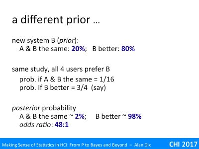
Now let’s imagine a slightly different prior where you are a little more confident in your new design. You think it four times more likely that you have managed to produce a better design than that you have made no difference (you are still modest enough to admit you may have done it badly!). Codified as a prior probability this gives us:
prior probability A & B are the same: 20%
prior probability B is better: 80%
The experimental results is exactly the same, but because the prior beliefs are different the posterior probability distribution is also different:
posterior probability A & B are the same: ~2%
posterior probability B is better: ~98%
The odds ratio is 48:1, which would be considered an overwhelmingly positive result; you would definitely conclude that system B is better.
Here the same study data leads to very different conclusions depending on the prior probability distribution. in other words your prior belief.
On the one hand this is a good thing, it precisely captures the difference between the situations where you toss the coin out of your pocket compared to the showman at the street market.
On the other hand, this also shows how sensitive the conclusions of Bayesian analysis are to your prior expectations. It is very easy to fall prey to confirmation bias, where the results of the analysis merely rubber stamp your initial impressions.

As is evident Bayesian inference can be really powerful in a variety of settings. As a statistical tool however, it is evident that the choice of prior is the most critical issue.
how do you get the prior?
Sometimes you have strong knowledge of the prior probability, perhaps based on previous similar experiments. However, this is more commonly the case for its use in internal algorithms, it is less clear in more typical usability settings such as the comparison between two systems. In these cases you are usually attempting to quantify your expert judgement.
Sometimes the evidence from the experiment or study is s overwhelming that it doesn’t make much difference what prior you choose … but in such cases hypothesis testing would give very high significance levels (low p values!), and confidence intervals very narrow ranges. It is nice when this happens, but if this were always the case we would not need the statistics!
Another option is to be conservative in your prior. The first example we gave was very conservative, giving the new system a low probability of success. More commonly a uniform prior is used, giving everything the same prior probability. This is easy when there a small number of distinct possibilities, you just make them equal, but a little more complex for unbounded value ranges, where often a Cauchy distribution is used … this is bell shaped a bit like the Normal distribution but has fatter edges, like an egg with more white.
In fact, if you use a uniform prior than the results of Bayesian statistics are pretty much identical to traditional statistics, the posterior is effectively the likelihood function, and the odds ratio is closely related to the significance level.
As we saw, if you do not use a uniform prior, or a prior based on well-founded previous research, you have to be very careful to avoid confirmation bias.
handling multiple evidence
Bayesian methods are particularly good at dealing with multiple independent sources of evidence; you simply apply the technique iteratively with the posterior of one study forming the prior to the next. However, you do need to be very careful that the evidence is really independent evidence, or apply corrections if it is not.
Imagine you have applied Bayesian statistics using the task completion times of an experiment to provide evidence that system B is better than system A. You then take the posterior from this study and use it as the prior applying Bayesian statistics to evidence from an error rate study. If these are really two independent studies this is fine, but of this is the task completion times and error rates from the same study then it is likely that if a participant found the task hard on one system they will have both slow times and more errors and vice versa – the evidence is not independent and your final posterior has effectively used some of the same evidence twice!
internecine warfare
Do be aware that there has been an on-going, normally good-natured, debate between statisticians on the relative merits of traditional and Bayesian statistics for at least 40 years. While Bayes Rule, the mathematics that underlies Bayesian methods, is applied across all branches of probability and statistics, Bayesian Statistics, the particular use for statistical inference, has always been less well accepted, the Cinderella of statistics.
However, algorithmic uses of Bayesian methods in machine learning and AI have blossomed over recent years, and are widely accepted and regarded across all communities.