 Many statistical tests depend on the idea of outcomes that are the same or worse than the one you have observed. For example, if you have the difference in response times between two systems is 5.7 seconds, then 5.8, 6, 23 seconds are all ‘the same or worse’, equally or more surprising. For numeric values this is fairly straightforward, but can be more complex when looking at different sorts of patterns in data. This is critical when you are making ‘post-hoc hypotheses’, noticing some pattern in the data and then trying to verify whether it is a real effect or simple chance.

You have got hold of the stallholder’s coin and wondering if it is fair or maybe weighted in some way.
Imagine you toss it 10 times and get the sequence: THTHHHTTHH
Does that seem reasonable?
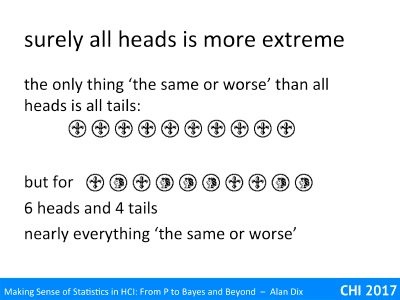
What about all heads? HHHHHHHHHH
In fact, if the coin is fair the probability of any sequence of heads and tails is the same: 1 in 1024
Prob( THTHHHTTHH ) = 1/ 210 ~ 0.001
Prob( HHHHHHHHHH ) = 1/ 210 ~ 0.001
The same would be true of a pack of cards. There are 52! Different ways a pack of cards can come out (Note. 52! Is 52 factorial, the product of all the numbers up to 52 = 52x51x50 … x3x2x1), approximately the number of atoms in our galaxy. Each order is equally likely on a wells shuffled pack, so any pack you pick up is incredibly unlikely.
However, this goes against our intuition that some orders of cards, some patterns of coin tosses are more special than others.
This is where we need to have an idea of things that are similar or equally surprising to each other.
For the line of 10 heads, the only thing equally surprising would be a line of 10 tails. However for the pattern THTHHHTTHH, with 6 heads and 4 tails in a pretty unsurprising order (not even all the heads together), pretty much any other order s equally or more surprising, indeed if you are thinking about a fair coin, arguably the only thing less surprising is exactly five of each.
This idea of same or worse is relatively straightforward for numeric data such as completion time in an experiment, or number of heads in coin tosses.
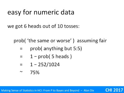
We got 6 heads out of 10 tosses, so that 6, 7, 8, 9, 10 heads would be equally or more surprising, as would 6,7,8,9,10 tails.
So …
prob ( ‘the same or worse’ ) assuming fair
= prob ( anything but 5H 5T )
= 1 – prob ( 5exactly 5 heads )
= 1 – 252/1024
~ 75%
Yep, the pattern THTHHHTTHH was not particularly surprising!

Lets look at another example, say it had been 9 heads and one tail.
Now 10 heads, or 9 tails, or 10 tails would all be equally or more surprising.
So …
prob ( ‘the same or worse’ ) assuming fair
= prob ( 9 heads ) + prob ( 10 heads )
+ prob ( 9 tails ) + prob ( 10 tails )
= 10/1024 + 1/1024 + 10/1024 + 1/1024
= 22/1024
~ 2%
So yes, 9 heads is starting to look more surprising, but is it enough to call the stallholder out for cheating?
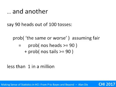
As a final example, imagine 90 heads out of 100 tosses – the same proportion, but more tosses, therefore you expect things to ‘average out’ more.
Here the things that are equally or more surprising are 90 or more heads or 90 or more tails.
prob ( ‘the same or worse’ ) assuming fair
= prob ( nos heads >= 90 ) + prob ( nos tails >= 90 )
less than 1 in a million
The maths for this gets a little more complicated, but turns out to be less than one in a million. If this were a Wild West film this is the point the table would get flung over and the shooting start!
For continuous distributions, such as task completion times, the principle is the same. The maths to work out the probabilities gets harder still, but here you just look up the numbers in a statistical table, or rely on R or SPSS to wok it out for you.
For example, you measure the average task completion time for ten users of system A as 117.3 seconds and for ten users of system B it is 98.1 seconds. On average for the participants in your user test system B was 18.2 seconds faster. Can you conclude that your newly designed system B is indeed faster to use?
Just as with the coin tosses, the probability of a precisely 18.2 second difference is vanishingly small, it could be 18.3 or 18.1, or so many possible values. Indeed, even if the systems were identical, the probability of the difference being precisely zero, or 0.1 seconds, or 0.2 seconds are all still pretty tiny. Instead you look at the probability (given the systems are the same) that the difference is 18.2 or greater.

For numeric values, the only real complication is whether you want a one or two tailed test. In the case of checking whether the coin is far, you would be equally upset if it had been weighted in some way in either direction, hence you look at both sides equally and work out (for the 90 heads out of 100): prob (nos heads >=90) + prob( nos tails >= 90).
However, for the response time, you probably only care about your new system being faster than the old one. So in this case you would only look at the probability of the time difference being >=18.2, and not bother about it being larger in the opposite direction.
Things get more complex in various forms of combinatorial data, for example, friendship circles in network data. Here what it means to be the ‘same or worse’ can be far more difficult.
As an example of this kind of complexity, we’ll return to playing cards. Recall as many ways to shuffle the pack as atoms in the galaxy.
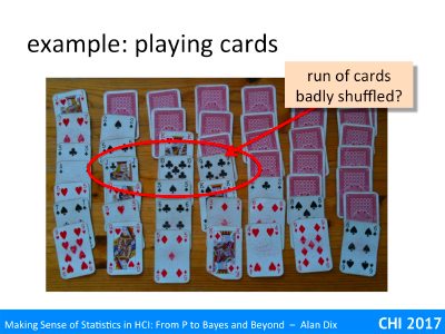
I sometimes play a variety of ‘patience’ (a solitaire card game) which involves laying out a 7×7 grid with the lower left triangle exposed and the upper right face down.
One day I was dealing these out and noticed that three consecutive cards had been jack of clubs, 10 of clubs, 9 of clubs.
My first thought was that I had not shuffled the cards well and this pattern was due to some systematic effects from a previous card game. However, I then realised that the previous game would not lead to sequences of cards in suit.
So what was going on? Remembering the rain drops in the Plains of Nali, is this chance or an omen?
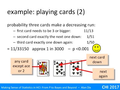
Let’s look a little more closely. If you deal three cards in a row, what is the probability it will be a decreasing sequence?
Well, the first card can be anything except an ace or a 2, that is 44 out of 52 cards, or 11/13.
After this the second and third cards are precisely determined by the first card, so have probability of 1/51 and 1/50 respectively.
Overall the probability f three cards being in a downward run in suit is 11/33350, or about 1 in 3000 … pretty unlikely and if it were doing statistics after a usability experiment you would get pretty excited with p <0.0001

However, that is not the end of the story. I would have been equally surprised if it had been an ascending, or if the run had been anywhere amongst the visible cards where there are 15 possible start positions for a run of three. So, our probability of it being a run up or down in any of these start positions is now 30 x 11 / 33350 or about 1 in a 100.
But then there are also vertical runs up and down the cards, or perhaps runs of the same number from different suits that would also be equally surprising.
Finally how many times do I play the game? I probably only notice when there is something interesting (cherry picking), suddenly my run of three does not looks so surprising.
In some ways noticing the jack, ten, nine run was a bit like a post-hoc hypothesis.
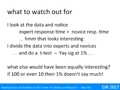
You have run your experiment, looked at the data and the notice that it looks as though expert response time is slower than novice response time. This looks interesting, so you follow this up with a formal statistical test. You divide the data into novice and expert calculate averages, do the sums and and it comes out significant at 1%.
Yay, you have found out something … or have you?
What else would have been equally interesting that you might have noticed, age effects, experience, exposure to other kinds of software, those wearing glasses vs. those with perfect visions?
Remember your Bonferroni correction, if there are 10 things that would have been equally surprising, your 1% statistical significance is really only equivalent to 10%, which may be just plain chance.
Think back to the raindrops patterns on the Plain of Nali. One day’s rainfall included three drops is an almost straight line, but turned out to be an entirely random fall pattern. You notice the three drops in a line, but how many lots of three are there, how close to a line before you call it straight? Would small triangles, or squares have been equally surprising.
In an ideal (scientific) world, you would use patterns you notice in data as hypotheses for a further round of experiments … but often that is not possible and you need to be able to both spot patterns and make tests on their reliability on the same data.
One way to ease this is to visualise a portion of the data and then check it on the rest – this is similar to techniques used in machine earning. However, again that may not always be possible.
So, if you do need to make post-hoc hypotheses, try to make an assessment of what other things would ‘similar or more surprising’ and use this to help decide whether you are just seeing random patterns in the wild-slung stars.